An introduction to the EJSCREENbatch tool
A.R. El-Khattabi, Morgan Teachey & Adam Theising
2023-08-24
EJSCREENbatch.RmdEnvironmental justice (EJ) analyses summarize demographics of local populations and environmental burden in order to measure the differential impacts that environmental policy decisions may have on affected communities. It is often helpful for regulators, analysts, and citizen communities to be able to assess impacts across many affected areas at once, allowing for comparison between communities and across regulatory actions. To streamline initial screening-level EJ analysis efforts, this package was developed to leverage national demographic and environmental datasets made available through the U.S. Environmental Protection Agency. Specifically, it allows users to analyze EJ summary statistics for an unlimited number of locations (coordinates, polygons, or water features) and produces customized figures and maps based on user specifications.
The EJSCREENbatch R package primarily relies on data provided by EJSCREEN, a mapping and screening tool maintained by EPA that provides demographic and environmental impact data on the Census Block Group (CBG) level for the United States. For information on how these data were prepared, refer to the EJSCREEN Technical Information Guidance.
This package also draws CBG-level demographic data from the Census Bureau’s American Community Survey (ACS) using the tidycensus R package.
Getting started
To access the latest version of the package, simply install from the EPA’s Github Repo using the devtools package:
# Import EJSCREENbatch package
library(devtools)
install_github(repo = "USEPA/EJSCREENbatch")
Next load the package (and others essential to this vignette):
Users should note that when the package is installed and certain functions are called, EJSCREEN and ACS data are downloaded and saved to the package’s library folder. For users that are hyper-conscious of local disk space, making a default EJfunction() call using the most recent releases of EJSCREEN/ACS data will locally save files that are roughly 1GB in size. For users who intend to perform screening analyses using older or multiple vintages of the EJSCREEN/ACS data, more or less disk space may be required.
Input data requirements
To run the tool, the user supplies input location data. Since this is a batch tool, the data can (and should!) include several input locations. These locations could be points in space (i.e. lat/long coordinates of an emitting facility), shapes (i.e. a set of linestrings representing streams/rivers or polygons representing wetlands, municipal boundaries, or air pollution plumes), or a waterbody identifier from the NHDPlus database (more on this below).
For illustrative purposes, we will work through this vignette using a dataset containing the latitude/longitude outfall coordinates for a set of meat and poultry processing (MPP) facilities in the Great Lakes region. These MPP outfalls feed directly into the US’s water network, and will serve as our “locations of interest” (LOIs) for the vignette’s sample EJ analysis.
### MPP facilities pulled from stable URL -- only those
mpp <- data.table::fread('https://ejscreenbatch-data.s3.amazonaws.com/dmr_mpp_facilities_2019.csv') %>%
  dplyr::filter(State %in% c('IL','IN','MI','OH','WI')) %>%
  sf::st_as_sf(coords = c('Facility Longitude', 'Facility Latitude'), crs = 4326)
One important technical item: location inputs must be fed into package functions either (1) as a simple feature (sf) data.frame for point/line/polygon shapes or (2) as a list of catchment common identifiers (COMIDs). See the sf package documentation for a primer on using spatial data in R and the nhdplusTools package for an overview of the catchment ID data structure.
For an illustrative sense of the geographies that will be screened, we map our location inputs below. In the next section, we draw spatial buffers around our locations to extract demographic and environmental data from EJSCREEN’s national database.
# Visualize locations of MPP facilities:
library(ggplot2)
ggplot() +
  geom_map(data = map_data('state') %>%
             dplyr::filter(region %in% c('illinois','indiana','michigan',
                                         'ohio','wisconsin')),
           map = map_data('state') %>%
             dplyr::filter(region %in% c('illinois','indiana','michigan',
                                         'ohio','wisconsin')),
           aes(x = long, y = lat, map_id = region),
           color = 'black',fill = NA) +
  geom_sf(data = mpp, color = 'red') +
  theme_minimal()
Compiling data: using EJfunction()
We now demonstrate the batch tool’s implementation. The foundation of the package is built around EJfunction(), which does the heavy lifting of data compilation, cleaning, and spatial computation. Based on the user-provided input data and options selected, buffers are drawn around locations, and data from EJSCREEN and the ACS are extracted and compiled for these areas.
The function’s primary role is the return of data.frames containing raw or summarized information. To provide meaningful and systematic comparisons across locations, the data.frames returned by EJfunction() report both national and state percentiles in addition to the raw demographic and environmental indicators.
An initial run
We begin by running a simple, EJ screening call on our set of location coordinates. EJfunction() accepts an sf data.frame as its data input.1
# A simple application of EJfunction()
my.EJ.data <-  EJfunction(mpp, buffer = 1, raster = T)
Note that this example function call may take several minutes to run on your machine depending on bandwidth and processor speed.
This proximity analysis draws a simple buffer of 1 mile (buffer = 1) around each location, and extracts/returns the raw EJSCREEN data for all CBGs that intersect with the buffer area. Under the default (and suggested) GIS method (raster = T), the function also returns a location-level summary data.frame that is similar in spirit to data returned from the EJSCREEN mapper or API. Our raster-based population weighting approach differs slightly from the EJSCREEN mapper’s because we rely on NASA’s SEDAC population grid, while EJSCREEN weights populations using Census block centroids. To align with the EJSCREEN population buffering approach, users can set the option (raster = F)
By default, this function returns 3 outputs to the user’s work environment:
my.EJ.data: a list of sub-objects that result from the screening (see below for details)
data.tog: an sf data.frame of the raw EJSCREEN and selected ACS demographic data for U.S. states and Puerto Rico.
raster_extract: a raster containing population counts for the North American continent.
data.tog and raster_extract are kept in memory by design to ease additional runs of EJfunction() should the user wish to fine-tune the analysis or to incorporate into custom data visualization or analyses as appropriate.
Census block group screening data
The object returned as my.EJ.data is a list of two data sub-objects:
names(my.EJ.data)
#> [1] "EJ.cbg.data" "EJ.loi.data"
First, CBG-level data for all block groups within the designated 1-mile buffer proximity are returned as EJ.cbg.data.2 CBGs are identified by the ID column; note that CBG population estimates in these data.frames are net of the population fraction that does not fall within any LOI’s buffer. This ensures that no double counting of population occurs should a user elect to sum up head counts across all impacted CBGs.
These data may be of interest to users for two reasons. (1) For users who want to characterize demographics and environmental characteristics across ALL LOIs, these data provide the opportunity to calculate statistics using population-weighted averaging or to sum the total population count living within the buffers of all the LOIs. (2) In cases where buffers are not overlapping, users can use the CBG-level data to develop a within-LOI, “neighborhood”-level analyses of populations that may be affected by policy. For a flavor of this data, we can explore the data.frame below, which has been filtered to include all block groups that fall within the distance buffers of MPP facilities in Wisconsin. The EJSCREEN variable names and definitions can be downloaded here.
Location of Interest screening data
Second, the location-level summaries are returned as EJ.loi.data. The LOI-level information here is analogous to the report returned from EJSCREEN’s online point-and-click mapper interface. Here, rather than compiling results for a single location, the data is returned in a tidy data.frame format for a batch of locations.
Each location is uniquely identified by the variable shape_ID.The data.frame includes national and state percentiles, as well as the population-weighted raw values for each EJSCREEN indicator and key demographic variables from the ACS. Here, we explore the summary return for each of the MPP facilities.
Adjusting user-selected options
The user is able to specify several alternative settings while compiling data with EJfunction(). These include:
- The buffer distance(s) within which to select proximate CBGs. Users can modify these distances (in miles) using the buffer argument. Input value(s) must be numeric and can be a vector if the user is interested in running analyses at several bandwidths.
# An example run with multiple buffer distances:
my.EJ.data.multibuffer <- EJfunction(LOI_data = mpp,
buffer = c(1,3,5))- The buffer GIS method used to apportion population for CBGs that overlap the LOI buffer’s boundary. Users specify this via the raster argument. The default setting is raster = T. This package is currently built to use NASA’s Socioeconomic Data and Application Center (SEDAC) 1km x 1km raster. The package’s buffering method relies on the 2010 vintage of the population count raster for all EJSCREEN vintages from 2021 or earlier, and the 2020 vintage in more recent years.
The alternative is to set this option to raster = F: doing so will result in use of the EJSCREEN Mapper’s methodology. EJfunction() will download census block centroid coordinates and use them to calculate the fraction of a boundary CBG’s population that falls within the LOI’s buffer. This fraction will then be used to population-weight demographic and environmental statistics as displayed in EJ.loi.data.
# An example run using the census block centroids to apportion buffer population.
my.EJ.data.block <- EJfunction(LOI_data = mpp,
                                   buffer = 1,
raster = F)- The data vintage used in the analysis, for cases when a user would like to perform a retrospective screening using older versions of the EJSCREEN and corresponding ACS data. This option is set with the data_year parameter using a numeric value. Currently, EJSCREENbatch allows for all vintages 2020 and later.
# An example run using EJSCREEN data from 2021.
my.EJ.data.2021 <- EJfunction(LOI_data = mpp,
                               buffer = 1,
data_year = 2021)- The state screen, for cases when a user wants to restrict analysis to a single state. This is set with the state argument, using the state’s designated two letter code.
# An example run restricting the screening only to the state of WI.
my.EJ.data.state <- EJfunction(LOI_data = mpp,
                               buffer = 1,
                               state = 'WI')
Water-based EJ screening analysis
The previous screening analyses using EJfunction() can also be completed using water-feature-based buffering. This package leverages the surface water network established in the National Hydrology Dataset (NHD), which incorporates the NHD, the National Elevation Dataset, and the National Watershed Boundary Dataset. Flowlines and catchments (watersheds) in this context therefore refer those established in the NHDPlusV2 (medium resolution). Users should note that these catchments are smaller in area than HUC12s.
To leverage this package’s water-based screening capabilities, users can supply either an sf data.frame of point coordinates or a list of catchment IDs (COMIDs) to the EJWaterReturnCatchmentBuffers() function.
Creating flowline shapes with an sf data.frame
Using our MPP outfall data, for example, we can call the following script in order to return an sf data.frame of flowlines shapes reaching 25 miles downstream of the outfalls.
mpp.flowlines <- EJWaterReturnCatchmentBuffers(mpp,
                              ds_us_mode = 'DM',
                              ds_us_dist = 25)
Underneath the hood, this function identifies catchments that lie within a specified distance up- or downstream (in river miles) of these starting locations. The function then creates a shapefile of each starting location’s associated flowline through these catchments. The user can modify two parameters: ds_us_dist is set as a numeric value to determine the distance down- or upstream that the flowline should run. ds_us_mode is set to determine whether the flowline shape returned should run downstream along the main stem (‘DM’), downstream including all diversions (‘DD’), upstream along the main stem (‘UM’) or upstream along all tributaries (‘UT’).
The returned list from EJWaterReturnCatchmentBuffers() contains 2 items: flowline_geoms and nhd_comids. The former is an sf data.frame, containing the user’s original input data with updated linestring geometries for each LOI’s flowline. The latter is a list of COMIDS through which each LOI passes. We envision that these COMID lists could be highly useful for supplemental analyses using other EPA water data products that are built on the NHDPlus network.
To illustrate the returned output, the flowlines for MPP facilities in the Great Lakes Region are mapped in the code block below:
ggplot() +
  geom_map(data = map_data('state') %>%
             dplyr::filter(region %in% c('illinois','indiana','michigan',
                                         'ohio','wisconsin')),
           map = map_data('state') %>%
             dplyr::filter(region %in% c('illinois','indiana','michigan',
                                         'ohio','wisconsin')),
           aes(x = long, y = lat, map_id = region),
           color = 'black',fill = NA) +
  geom_sf(data = mpp.flowlines$flowline_geoms,
          color = 'blue',
          size = 3) +
  geom_sf(data = mpp,
          color = 'darkblue') +
  theme_minimal()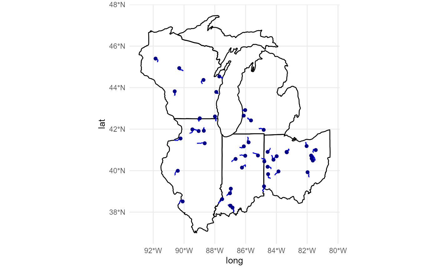
The dark blue points on the map represent the original coordinates in the MPP dataset; the lighter blue flowlines moving away from those points show the resulting linestring geometry produced in the output.
With this sf data.frame of flowline geometries (mpp.flowlines$flowline_geoms) in hand, it is now straightforward to call EJfunction() and return the environmental and demographic screening data for buffered areas 25 miles downstream of the MPP outfalls:
my.EJ.data.flowlines <- EJfunction(mpp.flowlines$flowline_geoms, buffer = 1, raster = T)The code block above draws a 1-mile buffer around the flowlines. The list of data.frames returned by EJfunction() are identical in structure to those shown above. It is worthwhile to explore the differences in demographic/environmental characteristics that result from taking a water-based buffering approach rather than a conventional circular buffer.
Creating flowline shapes with COMIDs
Lastly, it is possible to successfully call EJWaterReturnCatchmentBuffers() on non-sf data.frames in one specific case. If a user wishes to run a water-based screening analysis and has a data.frame with a “comid” column that holds (numeric) COMIDs for each LOI, the function will successfully return downstream flowlines and COMID lists.
Interactive mapping
For users that would like to explore their spatial data visually, the EJMaps() function creates an interactive map of the U.S. that displays the user’s locations of interest. Points/lines/polygons are shaded based on the number of indicators above a screening percentile threshold, allowing users to easily identify locations that may be good candidates for outreach efforts and/or further quantitative or qualitative analysis. The map’s interactive, point and click functionality also renders pop-up tables that share summary data for locations of interest. Values presented in the pop-up table are percentiles, meant to ease comparison in a national or state-level context.
EJMaps(input_data = my.EJ.data.flowlines,
       geography = 'US',
       indic_option = 'total',
       facil_name = 'Facility Name')[[1]]
#> Joining with `by = join_by(shape_ID)`
The indic_option parameter controls whether EJMaps()’s color shading scheme summarizes environmental or demographic indicators separately or summarizes all indicators together; the geography parameter designates whether national or state percentiles are used to compare against the threshold. The default threshold is set at 80, as suggested in the EJSCREEN technical guidance, but users can modify this threshold to suit their mapping needs. If the user’s input data includes a column that identifies LOIs (e.g. facility or location names), the facil_name parameter can be set equal to the column’s name (in string format).
Please note that this map visualization is a simple starting point for a regulatory screening analysis and that users are highly encouraged to produce their own figures and tables tailored to their locations of interest.
Using the EJSCREEN API
Finally, the EJSCREENbatch package has a canned function that allows users to make direct calls to the EJSCREEN API using an sf data.frame and numeric distance (in miles) as inputs. This function loops through API calls, LOI-by-LOI, mirroring the batch ethos used in EJfunction().
my.EJ.data.api <- EJSCREENBufferAPI(input_data = mpp.flowlines$flowline_geoms,
                                    dist = 1)
The function, EJSCREENBufferAPI(), will return a data.frame containing the full “firehose” of variables provided by EJSCREEN. This includes all the standard EJ environmental and demographic indicators, as well as CBG-level indicators about health disparities, climate change burden, critical service gaps, and a richer set of demographic information. Over 500 variables are returned by the API; see the EJSCREEN map descriptions for more details.
names(my.EJ.data.api)
#>   [1] "NPDES Permit Number"          "FRS ID"
#>   [3] "Facility Name"                "City"
#>   [5] "County"                       "State"
#>   [7] "HUC 12 Code"                  "Watershed Name"
#>   [9] "SIC Code"                     "Pollutant Name"
#>  [11] "Substance Registry System ID" "CAS Number"
#>  [13] "Average Daily Flow (MGD)"     "Major/Non-Major Status"
#>  [15] "Contains Potential Outliers?" "Total Pounds (lb/yr)"
#>  [17] "Total TWPE (lb-eq/yr)"        "Link to DFR"
#>  [19] "TOTALPOP"                     "NUM_MINORITY"
#>  [21] "WHITE"                        "BLACK"
#>  [23] "AMERIND"                      "ASIAN"
#>  [25] "HAWPAC"                       "OTHER_RACE"
#>  [27] "TWOMORE"                      "HISP"
#>  [29] "NHWHITE"                      "NHBLACK"
#>  [31] "NHAMERIND"                    "NHASIAN"
#>  [33] "NHHAWPAC"                     "NHOTHER_RACE"
#>  [35] "NHTWOMORE"                    "MALES"
#>  [37] "FEMALES"                      "AGE_LT5"
#>  [39] "AGE_LT18"                     "AGE_GT17"
#>  [41] "AGE_GT64"                     "HSHLD_INCOME"
#>  [43] "LESS_15"                      "15_20"
#>  [45] "25_50"                        "50_75"
#>  [47] "PLUS75"                       "HSUNITS"
#>  [49] "HSUNITS_PRE1950"              "OCCHU"
#>  [51] "OWNHU"                        "RENTHU"
#>  [53] "TOTAL_PLUS25"                 "NO_HS"
#>  [55] "NO_DIPLOMA"                   "HS_GRAD"
#>  [57] "SOME_COLLEGE"                 "ASSOC_DEGREE"
#>  [59] "BACH_DEGREE"                  "LAN_UNIVERSE"
#>  [61] "ENG_ONLY"                     "NON_ENG_HOME"
#>  [63] "ENG_VERY_WELL"                "ENG_WELL"
#>  [65] "ENG_NOT_WELL"                 "ENG_NOT"
#>  [67] "ENG_LESS_WELL"                "ENG_LESS_VERYWELL"
#>  [69] "AREALAND"                     "AREAWATER"
#>  [71] "LINGISO"                      "HLI_SPANISH_LI"
#>  [73] "HLI_IE_LI"                    "HLI_API_LI"
#>  [75] "HLI_OTHER_LI"                 "HH_BPOV"
#>  [77] "EMP_STAT_UNIVERSE"            "EMP_STAT_IN_LF"
#>  [79] "EMP_STAT_NOT_IN_LF"           "EMP_STAT_UNEMPLOYED"
#>  [81] "LOWINC"                       "POV_UNIVERSE_FRT"
#>  [83] "DISABILITY"                   "DISAB_UNIVERSE"
#>  [85] "M_TOTALPOP"                   "M_NUM_MINORITY"
#>  [87] "M_WHITE"                      "M_BLACK"
#>  [89] "M_AMERIND"                    "M_ASIAN"
#>  [91] "M_HAWPAC"                     "M_OTHER_RACE"
#>  [93] "M_TWOMORE"                    "M_HISP"
#>  [95] "M_NHWHITE"                    "M_NHBLACK"
#>  [97] "M_NHAMERIND"                  "M_NHASIAN"
#>  [99] "M_NHHAWPAC"                   "M_NHOTHER_RACE"
#> [101] "M_NHTWOMORE"                  "M_MALES"
#> [103] "M_FEMALES"                    "M_AGE_LT5"
#> [105] "M_AGE_LT18"                   "M_AGE_GT17"
#> [107] "M_AGE_GT64"                   "M_HSHLD_INCOME"
#> [109] "M_PER_CAP_INC"                "M_LESS_15"
#> [111] "M_15_20"                      "M_25_50"
#> [113] "M_50_75"                      "M_PLUS75"
#> [115] "M_HSUNITS"                    "M_HSUNITS_PRE1950"
#> [117] "M_OCCHU"                      "M_OWNHU"
#> [119] "M_RENTHU"                     "M_TOTAL_PLUS25"
#> [121] "M_NO_HS"                      "M_NO_DIPLOMA"
#> [123] "M_HS_GRAD"                    "M_SOME_COLLEGE"
#> [125] "M_ASSOC_DEGREE"               "M_BACH_DEGREE"
#> [127] "M_LAN_UNIVERSE"               "M_ENG_ONLY"
#> [129] "M_NON_ENG_HOME"               "M_ENG_VERY_WELL"
#> [131] "M_ENG_WELL"                   "M_ENG_NOT_WELL"
#> [133] "M_ENG_NOT"                    "M_ENG_LESS_WELL"
#> [135] "M_ENG_LESS_VERYWELL"          "M_LINGISO"
#> [137] "M_HLI_SPANISH_LI"             "M_HLI_IE_LI"
#> [139] "M_HLI_API_LI"                 "M_HLI_OTHER_LI"
#> [141] "M_HH_BPOV"                    "M_EMP_STAT_UNIVERSE"
#> [143] "M_EMP_STAT_IN_LF"             "M_EMP_STAT_NOT_IN_LF"
#> [145] "M_EMP_STAT_UNEMPLOYED"        "M_LOWINC"
#> [147] "M_POV_UNIVERSE_FRT"           "M_DISABILITY"
#> [149] "M_DISAB_UNIVERSE"             "P_BACH_DEGREE"
#> [151] "P_TOTAL_PLUS25"               "P_NO_DIPLOMA"
#> [153] "P_ASSOC_DEGREE"               "P_HS_GRAD"
#> [155] "P_NO_HS"                      "P_SOME_COLLEGE"
#> [157] "P_ENG_LESS_VERYWELL"          "P_NON_ENG_HOME"
#> [159] "P_ENG_WELL"                   "P_ENG_LESS_WELL"
#> [161] "P_ENG_NOT_WELL"               "P_LAN_UNIVERSE"
#> [163] "P_ENG_ONLY"                   "P_ENG_NOT"
#> [165] "P_DISAB_UNIVERSE"             "P_DISABILITY"
#> [167] "P_ENG_VERY_WELL"              "P_PLUS75"
#> [169] "P_15_20"                      "P_50_75"
#> [171] "P_25_50"                      "P_HSHLD_INCOME"
#> [173] "P_LESS_15"                    "P_HLI_IE_LI"
#> [175] "P_HLI_OTHER_LI"               "P_HLI_API_LI"
#> [177] "P_LINGISO"                    "P_HLI_SPANISH_LI"
#> [179] "P_EMP_STAT_UNIVERSE"          "P_EMP_STAT_IN_LF"
#> [181] "P_EMP_STAT_NOT_IN_LF"         "P_EMP_STAT_UNEMPLOYED"
#> [183] "P_LOWINC"                     "P_POV_UNIVERSE_FRT"
#> [185] "POP_DEN"                      "PCT_MINORITY"
#> [187] "PCT_AREALAND"                 "PCT_AREAWATER"
#> [189] "ONERACE"                      "M_ONERACE"
#> [191] "TOTAL_POP"                    "TOTAL_NHPOP"
#> [193] "P_TOTALPOP"                   "P_ONERACE"
#> [195] "P_WHITE"                      "P_BLACK"
#> [197] "P_AMERIND"                    "P_ASIAN"
#> [199] "P_HAWPAC"                     "P_OTHER_RACE"
#> [201] "P_TWOMORE"                    "P_HISP"
#> [203] "P_NHWHITE"                    "P_NHBLACK"
#> [205] "P_NHAMERIND"                  "P_NHASIAN"
#> [207] "P_NHHAWPAC"                   "P_NHOTHER_RACE"
#> [209] "P_NHTWOMORE"                  "P_MALES"
#> [211] "P_FEMALES"                    "P_AGE_LT5"
#> [213] "P_AGE_LT18"                   "P_AGE_GT17"
#> [215] "P_AGE_GT64"                   "M_TOTAL_POP"
#> [217] "P_TOTAL_POP"                  "TOTAL_HSHLD_TENURE"
#> [219] "OWN_OCCUPIED"                 "RENT_OCCUPIED"
#> [221] "M_TOTAL_HSHLD_TENURE"         "M_OWN_OCCUPIED"
#> [223] "M_RENT_OCCUPIED"              "HSHOLDS"
#> [225] "P_OWN_OCCUPIED"               "P_RENT_OCCUPIED"
#> [227] "P_TOTAL_HSHLD_TENURE"         "PER_CAP_INC"
#> [229] "LIFEEXP"                      "P_EDU_LTHS"
#> [231] "P_HSUNITS_PRE1950"            "P_LIMITED_ENG_HH"
#> [233] "LAN_UNIVERSE2"                "ENGLISH"
#> [235] "SPANISH"                      "FRENCH"
#> [237] "GERMAN"                       "RUS_POL_SLAV"
#> [239] "OTHER_IE"                     "KOREAN"
#> [241] "CHINESE"                      "VIETNAMESE"
#> [243] "TAGALOG"                      "OTHER_ASIAN"
#> [245] "ARABIC"                       "OTHER"
#> [247] "NON_ENGLISH"                  "M_LAN_UNIVERSE2"
#> [249] "M_ENGLISH"                    "M_SPANISH"
#> [251] "M_FRENCH"                     "M_GERMAN"
#> [253] "M_RUS_POL_SLAV"               "M_OTHER_IE"
#> [255] "M_KOREAN"                     "M_CHINESE"
#> [257] "M_VIETNAMESE"                 "M_TAGALOG"
#> [259] "M_OTHER_ASIAN"                "M_ARABIC"
#> [261] "M_OTHER"                      "M_NON_ENGLISH"
#> [263] "P_KOREAN"                     "P_TAGALOG"
#> [265] "P_OTHER"                      "P_LAN_UNIVERSE2"
#> [267] "P_OTHER_ASIAN"                "P_ARABIC"
#> [269] "P_GERMAN"                     "P_RUS_POL_SLAV"
#> [271] "P_OTHER_IE"                   "P_VIETNAMESE"
#> [273] "P_CHINESE"                    "P_ENGLISH"
#> [275] "P_NON_ENGLISH"                "P_SPANISH"
#> [277] "P_FRENCH"                     "RAW_D_PEOPCOLOR"
#> [279] "RAW_D_INCOME"                 "RAW_D_LESSHS"
#> [281] "RAW_D_LING"                   "RAW_D_UNDER5"
#> [283] "RAW_D_OVER64"                 "RAW_D_UNEMPLOYED"
#> [285] "RAW_D_LIFEEXP"                "RAW_D_DEMOGIDX2"
#> [287] "RAW_D_DEMOGIDX5"              "RAW_E_LEAD"
#> [289] "RAW_E_DIESEL"                 "RAW_E_CANCER"
#> [291] "RAW_E_RESP"                   "RAW_E_TRAFFIC"
#> [293] "RAW_E_NPDES"                  "RAW_E_NPL"
#> [295] "RAW_E_RMP"                    "RAW_E_TSDF"
#> [297] "RAW_E_O3"                     "RAW_E_PM25"
#> [299] "RAW_E_UST"                    "RAW_E_RSEI_AIR"
#> [301] "S_D_PEOPCOLOR"                "S_D_INCOME"
#> [303] "S_D_LESSHS"                   "S_D_LING"
#> [305] "S_D_UNDER5"                   "S_D_OVER64"
#> [307] "S_D_UNEMPLOYED"               "S_D_LIFEEXP"
#> [309] "S_D_DEMOGIDX2"                "S_D_DEMOGIDX5"
#> [311] "S_E_LEAD"                     "S_E_DIESEL"
#> [313] "S_E_CANCER"                   "S_E_RESP"
#> [315] "S_E_TRAFFIC"                  "S_E_NPDES"
#> [317] "S_E_NPL"                      "S_E_RMP"
#> [319] "S_E_TSDF"                     "S_E_O3"
#> [321] "S_E_PM25"                     "S_E_UST"
#> [323] "S_E_RSEI_AIR"                 "S_D_PEOPCOLOR_PER"
#> [325] "S_D_INCOME_PER"               "S_D_LESSHS_PER"
#> [327] "S_D_LING_PER"                 "S_D_UNDER5_PER"
#> [329] "S_D_OVER64_PER"               "S_D_UNEMPLOYED_PER"
#> [331] "S_D_LIFEEXP_PER"              "S_D_DEMOGIDX2_PER"
#> [333] "S_D_DEMOGIDX5_PER"            "S_E_LEAD_PER"
#> [335] "S_E_DIESEL_PER"               "S_E_CANCER_PER"
#> [337] "S_E_RESP_PER"                 "S_E_TRAFFIC_PER"
#> [339] "S_E_NPDES_PER"                "S_E_NPL_PER"
#> [341] "S_E_RMP_PER"                  "S_E_TSDF_PER"
#> [343] "S_E_O3_PER"                   "S_E_PM25_PER"
#> [345] "S_E_UST_PER"                  "S_E_RSEI_AIR_PER"
#> [347] "S_P2_LEAD"                    "S_P2_DIESEL"
#> [349] "S_P2_CANCER"                  "S_P2_RESP"
#> [351] "S_P2_TRAFFIC"                 "S_P2_NPDES"
#> [353] "S_P2_NPL"                     "S_P2_RMP"
#> [355] "S_P2_TSDF"                    "S_P2_O3"
#> [357] "S_P2_PM25"                    "S_P2_UST"
#> [359] "S_P2_RSEI_AIR"                "S_P5_LEAD"
#> [361] "S_P5_DIESEL"                  "S_P5_CANCER"
#> [363] "S_P5_RESP"                    "S_P5_TRAFFIC"
#> [365] "S_P5_NPDES"                   "S_P5_NPL"
#> [367] "S_P5_RMP"                     "S_P5_TSDF"
#> [369] "S_P5_O3"                      "S_P5_PM25"
#> [371] "S_P5_UST"                     "S_P5_RSEI_AIR"
#> [373] "N_D_PEOPCOLOR"                "N_D_INCOME"
#> [375] "N_D_LESSHS"                   "N_D_LING"
#> [377] "N_D_UNDER5"                   "N_D_OVER64"
#> [379] "N_D_UNEMPLOYED"               "N_D_LIFEEXP"
#> [381] "N_D_DEMOGIDX2"                "N_D_DEMOGIDX5"
#> [383] "N_E_LEAD"                     "N_E_DIESEL"
#> [385] "N_E_CANCER"                   "N_E_RESP"
#> [387] "N_E_TRAFFIC"                  "N_E_NPDES"
#> [389] "N_E_NPL"                      "N_E_RMP"
#> [391] "N_E_TSDF"                     "N_E_O3"
#> [393] "N_E_PM25"                     "N_E_UST"
#> [395] "N_E_RSEI_AIR"                 "N_D_PEOPCOLOR_PER"
#> [397] "N_D_INCOME_PER"               "N_D_LESSHS_PER"
#> [399] "N_D_LING_PER"                 "N_D_UNDER5_PER"
#> [401] "N_D_OVER64_PER"               "N_D_UNEMPLOYED_PER"
#> [403] "N_D_LIFEEXP_PER"              "N_D_DEMOGIDX2_PER"
#> [405] "N_D_DEMOGIDX5_PER"            "N_E_LEAD_PER"
#> [407] "N_E_DIESEL_PER"               "N_E_CANCER_PER"
#> [409] "N_E_RESP_PER"                 "N_E_TRAFFIC_PER"
#> [411] "N_E_NPDES_PER"                "N_E_NPL_PER"
#> [413] "N_E_RMP_PER"                  "N_E_TSDF_PER"
#> [415] "N_E_O3_PER"                   "N_E_PM25_PER"
#> [417] "N_E_UST_PER"                  "N_E_RSEI_AIR_PER"
#> [419] "N_P2_LEAD"                    "N_P2_DIESEL"
#> [421] "N_P2_CANCER"                  "N_P2_RESP"
#> [423] "N_P2_TRAFFIC"                 "N_P2_NPDES"
#> [425] "N_P2_NPL"                     "N_P2_RMP"
#> [427] "N_P2_TSDF"                    "N_P2_O3"
#> [429] "N_P2_PM25"                    "N_P2_UST"
#> [431] "N_P2_RSEI_AIR"                "N_P5_LEAD"
#> [433] "N_P5_DIESEL"                  "N_P5_CANCER"
#> [435] "N_P5_RESP"                    "N_P5_TRAFFIC"
#> [437] "N_P5_NPDES"                   "N_P5_NPL"
#> [439] "N_P5_RMP"                     "N_P5_TSDF"
#> [441] "N_P5_O3"                      "N_P5_PM25"
#> [443] "N_P5_UST"                     "N_P5_RSEI_AIR"
#> [445] "stateAbbr"                    "stateName"
#> [447] "epaRegion"                    "totalPop"
#> [449] "NUM_NPL"                      "NUM_TSDF"
#> [451] "NUM_WATERDIS"                 "NUM_AIRPOLL"
#> [453] "NUM_BROWNFIELD"               "NUM_TRI"
#> [455] "NUM_SCHOOL"                   "NUM_HOSPITAL"
#> [457] "NUM_CHURCH"                   "YESNO_TRIBAL"
#> [459] "YESNO_CEJSTDIS"               "YESNO_IRADIS"
#> [461] "YESNO_AIRNONATT"              "YESNO_IMPWATERS"
#> [463] "YESNO_HOUSEBURDEN"            "YESNO_TRANSDIS"
#> [465] "YESNO_FOODDESERT"             "centroidX"
#> [467] "centroidY"                    "statLayerCount"
#> [469] "statLayerZeroPopCount"        "weightLayerCount"
#> [471] "timeSeconds"                  "distance"
#> [473] "unit"                         "statlevel"
#> [475] "inputAreaMiles"               "placename"
#> [477] "RAW_HI_LIFEEXP"               "RAW_HI_LIFEEXPPCT"
#> [479] "RAW_HI_HEARTDISEASE"          "RAW_HI_ASTHMA"
#> [481] "RAW_HI_CANCER"                "RAW_HI_DISABILITYPCT"
#> [483] "RAW_CG_LIMITEDBBPCT"          "RAW_CG_NOHINCPCT"
#> [485] "RAW_CI_FLOOD"                 "RAW_CI_FLOOD30"
#> [487] "RAW_CI_FIRE"                  "RAW_CI_FIRE30"
#> [489] "S_HI_LIFEEXP_AVG"             "S_HI_LIFEEXPPCT_AVG"
#> [491] "S_HI_HEARTDISEASE_AVG"        "S_HI_ASTHMA_AVG"
#> [493] "S_HI_CANCER_AVG"              "S_HI_DISABILITYPCT_AVG"
#> [495] "S_CG_LIMITEDBBPCT_AVG"        "S_CG_NOHINCPCT_AVG"
#> [497] "S_CI_FLOOD_AVG"               "S_CI_FLOOD30_AVG"
#> [499] "S_CI_FIRE_AVG"                "S_CI_FIRE30_AVG"
#> [501] "S_HI_LIFEEXP_PCTILE"          "S_HI_LIFEEXPPCT_PCTILE"
#> [503] "S_HI_HEARTDISEASE_PCTILE"     "S_HI_ASTHMA_PCTILE"
#> [505] "S_HI_CANCER_PCTILE"           "S_HI_DISABILITYPCT_PCTILE"
#> [507] "S_CG_LIMITEDBBPCT_PCTILE"     "S_CG_NOHINCPCT_PCTILE"
#> [509] "S_CI_FLOOD_PCTILE"            "S_CI_FLOOD30_PCTILE"
#> [511] "S_CI_FIRE_PCTILE"             "S_CI_FIRE30_PCTILE"
#> [513] "N_HI_LIFEEXP_AVG"             "N_HI_LIFEEXPPCT_AVG"
#> [515] "N_HI_HEARTDISEASE_AVG"        "N_HI_ASTHMA_AVG"
#> [517] "N_HI_CANCER_AVG"              "N_HI_DISABILITYPCT_AVG"
#> [519] "N_CG_LIMITEDBBPCT_AVG"        "N_CG_NOHINCPCT_AVG"
#> [521] "N_CI_FLOOD_AVG"               "N_CI_FLOOD30_AVG"
#> [523] "N_CI_FIRE_AVG"                "N_CI_FIRE30_AVG"
#> [525] "N_HI_LIFEEXP_PCTILE"          "N_HI_LIFEEXPPCT_PCTILE"
#> [527] "N_HI_HEARTDISEASE_PCTILE"     "N_HI_ASTHMA_PCTILE"
#> [529] "N_HI_CANCER_PCTILE"           "N_HI_DISABILITYPCT_PCTILE"
#> [531] "N_CG_LIMITEDBBPCT_PCTILE"     "N_CG_NOHINCPCT_PCTILE"
#> [533] "N_CI_FLOOD_PCTILE"            "N_CI_FLOOD30_PCTILE"
#> [535] "N_CI_FIRE_PCTILE"             "N_CI_FIRE30_PCTILE"
#> [537] "geometry"
This function may be particularly useful in cases where only LOI-level screening data are needed. EJSCREEN’s API is not terribly fast, however, so users should expect a need for patience and plan to streamline the returned data.frame into more usable content for analytics.