rExpertQuery Cybertown Training

About Expert Query and rExpertQuery

Expert Query empowers users to access surface water quality data from the Assessment and TMDL Tracking and Implementation System (ATTAINS) encompassing Assessment decisions (under Clean Water Act Sections 303(d), 305(b), and 106) and Action data like Total Maximum Daily Loads (TMDLs), Advance Restoration Plans (ARPs), and Protection Approaches.

The tool supports querying and downloading data within and across organizations (states or tribes), such as querying all the data within an EPA region or all nutrient TMDLs nationally. It also allows users to download national ATTAINS data extracts.

rExpertQuery takes this a step further as its functions facilitate querying the Expert Query web services and importing the resulting data sets directly in to R for more detailed review and analysis.

It is crucial to be aware of certain complexities inherent in the data and querying process. Users are cautioned against direct comparisons between states due to differences in water quality standards and assessment methodologies. The summary and count examples provided here are intended to demonstrate potential uses of rExpertQuery and complementary R packages, but do not imply EPA’s endorsement of any specific summary or count method.

While Expert Query facilitates data querying, it lacks built-in summary capabilities. Users are encouraged to download and summarize data, but use caution when relying on row counts, as duplicate entries may occur. This complexity arises from multiple tables that have many-to-many relationships. Several examples of summarizing Expert Query data are included in this vignette. These examples use additional packages for data wrangling, mapping, visualizing and other tasks. Future rExpertQuery vignettes and functions may provide additional examples of how to summarize Expert Query data.

Installation

You must first have R and R Studio installed to use the rExpert Query (see instructions below if needed). rExpert Query is in active development, therefore we highly recommend that you update it and all of its dependency libraries each time you use the package.

You can install and/or update the rExpertQuery Package and all dependencies by running:

# install and load rExpertQuery
if (!"remotes" %in% installed.packages()) {
  install.packages("remotes")
}

remotes::install_github("USEPA/rExpertQuery", ref = "develop", dependencies = TRUE, force = TRUE)

## Using github PAT from envvar GITHUB_PAT. Use `gitcreds::gitcreds_set()` and unset GITHUB_PAT in .Renviron (or elsewhere) if you want to use the more secure git credential store instead.

## Downloading GitHub repo USEPA/rExpertQuery@develop

## 
## ── R CMD build ─────────────────────────────────────────────────────────────────
## * checking for file ‘/tmp/RtmpVpDgsh/remotes224d77840daf/USEPA-rExpertQuery-5f882fb/DESCRIPTION’ ... OK
## * preparing ‘rExpertQuery’:
## * checking DESCRIPTION meta-information ... OK
## * checking for LF line-endings in source and make files and shell scripts
## * checking for empty or unneeded directories
## Omitted ‘LazyData’ and ‘LazyDataCompression’ from DESCRIPTION
## * building ‘rExpertQuery_0.1.0.tar.gz’

## Installing package into '/home/runner/work/_temp/Library'
## (as 'lib' is unspecified)

library(rExpertQuery)

This vignette also requires additional packages which can be installed using the code chunk below:

# # list of additional required packages
#  demo.pkgs <- c("datasets", "data.table", "dplyr", "DT", "ggplot2", "httr", "leaflet", "maps", "plotly", "sf", "usdata", "usmap", "stringi")
# 
# # install additional packages not yet installed
#  installed_packages <- demo.pkgs %in% rownames(installed.packages())
#  
# if (any(installed_packages == FALSE)) {
#    install.packages(demo.pkgs[!installed_packages])
#  }

# load additional packages for this vignette
library(datasets)
library(data.table)
library(dplyr)
library(DT)
library(ggplot2)
library(httr)
library(leaflet)
library(maps)
library(plotly)
library(sf)
library(usdata)
library(usmap)
library(stringi)

As a final setup step, we will turn off scientific notation so that any catchment id numbers from our queries are displayed correctly.

# turn off scientific notation (for catchment ids)
options(scipen = 999)

API Key

Most of the rExpertQuery functions require an API key. Users can obtain their own by using Expert Query’s API Key Signup Form.

A screenshot of the web page to sign up for your Expert Query API Key

To run this vignette, we can use the following test key. Users should obtain their own API key if they will be using rExpertQuery to develop their own workflows.

# load test api  key
testkey <- "53BVce47MQ3KXKibjx35g4ojaDQGh8qWfbdO8cE0"

rExpert Query Functions

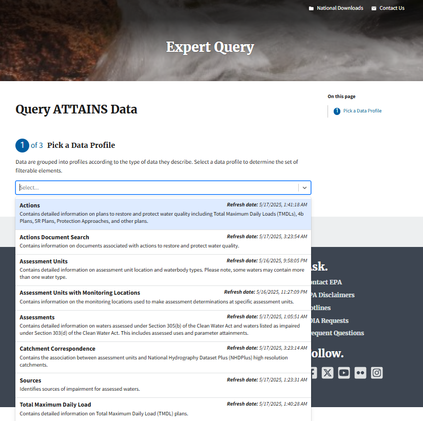
There are ten exported functions in rExpertQuery. The first eight allow users to query ATTAINS data via Expert Query web services. These are:

EQ_Actions() - queries and returns ATTAINS actions data
EQ_ActionsDocuments() - queries and returns ATTAINS Actions Documents, including a keyword search
EQ_Assessments() - queries and returns ATTAINS Assessments (default is for latest cycle)
EQ_AssessmentUnits() - queries and returns ATTAINS Assessment Units (default is for Active AUs)
EQ_AUsMLs() - queries and returns ATTAINS Assessment Units with Monitoring Location data
EQ_CatchCorr() - queries and returns ATTAINS Catchment Correspondence data (memory intensive)
EQ_Sources() - queries and returns ATTAINS Sources data
EQ_TMDLs() - queries and returns ATTAINS TMDL data

These first eight functions are analogous to the data profiles that can be queried through the Expert Query User Interface.

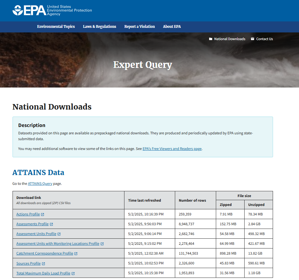
A screenshot of the Expert Query user interface with the dropdown menu open to display the profile options.

An additional function allows users to download the Expert Query National Extracts of ATTAINS data which are updated weekly. This function should be used when national data are desired or when a query designed in one of the previous eight functions would exceed the Expert Query web services limit of one millions rows. This function is:

EQ_NationalExtract() - returns national extract for Actions, Assessments, Assessment Units, Assessment Units with Monitoring Locations, Catchment Correspondence, Sources, or TMDLS based on user selection

The tenth function relies on ATTAINS web services to provide allowable domain values for some rExpertQuery parameters:

EQ_DomainValues() - returns domain values for some rExpertQuery function params

Demo Structure

In this session, we will use rExpertQuery functions, along with some common R packages for data wrangling and visualization to answer some commonly asked questions with Expert Query data. Members of the ATTAINS team will be monitoring the chat for questions. If there are many questions regarding a particular function, we may pause at the end of that function’s material to review. Otherwise, questions are welcome at the end of the demo as time permits or via e-mailing the ATTAINS team at attains@epa.gov.

EQ_NationalExtract

EQ_NationalExtract() provides an efficient method for importing the Expert Query National Extracts. This function requires one argument, “extract” to specify which of the National Extracts to download. The following examples show how to download the Assessments and Assessments with Monitoring Locations extracts. The extracts are all large files and some may not open in R if there is not enough memory available.

A screenshot of the Expert Query National Downloads web page

What is the most commonly reported impairment nationally?

After downloading the national assessments data, we’ll need to filter to include only the latest cycle. Next, we can filter for rows containing parameter causes, and summarize how many times each parameter was listed as a cause of impairment. The additional packages used to answer this question are dplyr (data manipulation) and DT (interface to DataTables library).
```
# import natioanl assessments profile
assessments.nat <- rExpertQuery::EQ_NationalExtract("assessments")
```
```
## [1] "EQ_NationalExtract: downloading Assessments Profile (Expert Query National Extract). It was last updated on May 31, 2025 at 02:22 AM UTC."
## [1] "EQ_NationalExtract: unzipping Assessments Profile (Expert Query National Extract)."
## [1] "EQ_NationalExtract: opening Assessments Profile (Expert Query National Extract)."
```
```
# filter for latest assessments
assessments.nat <- assessments.nat %>%
   dplyr::group_by(organizationId) %>%
    dplyr::slice_max(reportingCycle) %>%
    dplyr::select(-objectId) %>%
    dplyr::distinct() %>%
    dplyr::ungroup()

# count impairments
count.impair <- assessments.nat %>%
  # filter to retain only parameter causes
  dplyr::filter(parameterStatus == "Cause") %>%
  # subset data to find unique combinations
  dplyr::select(organizationId, assessmentUnitId, parameterName) %>%
  # remove duplicates
  dplyr::distinct() %>%
  # group by parameterName
  dplyr::group_by(parameterName) %>%
  # count listings for each parameterName
  dplyr::summarise(count = length(assessmentUnitId)) %>%
  # arrane in descending order
  dplyr::arrange(desc(count))

# create data table of impairment count results
DT::datatable(count.impair, options = list(pageLength = 10, scrollX = TRUE))
```
Which waters are impaired for SELENIUM nationally? Which states contain waters impaired for SELENIUM?

Again, we’ll use the national assessments data filtered to the latest cycle. Then we will filter for rows where the parameter is both selenium and listed as a cause. The additional packages used in this step are dplyr and DT.
```
# filter assessments data set for 
param.nat <- assessments.nat %>% 
  # filter for selenium and cause
  dplyr::filter(parameterName == "SELENIUM" &
                  parameterStatus == "Cause")

# data table of selenium impairments
DT::datatable(param.nat, options = list(pageLength = 5, scrollX = TRUE))
```
Then we can create a list of states that have at least one selenium impairment listed. We can also visualize this information on a map, with states containing selenium impairments filled in blue. To build this map, we first create a data frame with all 50 states and a “SeleniumImpairment” column populated with “yes” or “no” to indicate whether it has any listed selenium impairments.

In addition to dplyr, this code chunk also uses usdata (US demographic data), datasets (collection of data sets for use in R), usmap (US choropleth plotting) and ggplot2 (creating graphics).
```
# filter to create df of states that have at least one selenium impairment}
state.names.sel <- param.nat %>%
  # select state column from filtered df
  dplyr::select(state) %>%
  # retain only distinct values for state
  dplyr::distinct() %>%
  # change state abbreviation to full state name
  dplyr::mutate(state = usdata::abbr2state(state)) %>%
  # create a list from the df
  dplyr::pull()

# read in a list of all 50 state  names
state.names <- datasets::state.name

# create df with of all 50 state names
sel.map.data <- as.data.frame(state.names) %>%
  # rename state.name column to state
  dplyr::rename(state = state.names) %>%
  # create additional column to indicate if state has recorded selenium impairments ("yes") or not ("no")
  dplyr::mutate(SeleniumImpairment = factor(ifelse(state %in% state.names.sel,
                                            "yes", "no")))
```
```
# create map, specifying data and values
usmap::plot_usmap(
  regions = "state", data = sel.map.data,
  values = "SeleniumImpairment", color = "black"
) +
# fill states with selenium impairments with blue
  ggplot2::scale_fill_manual(
    values = c(`no` = "white", `yes` = "blue")
  ) +
# remove legend
  ggplot2::theme(legend.position = "none")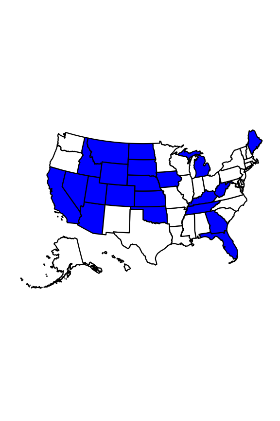
```
Fig 1. States with selenium listed as a cause of impairment for any waters are shown in blue.
Which waters have a TMDL and are fully supporting nationally?

Starting with the filtered data frame of latest cycle assessments, we can filter for Fully Supporting waters with an asssociatedActionType of “TMDL”. Again, we can use a combination of dplyr and DT, for data manipulation and creating a data table, respectively.
```
# filter national assessments to includ only Fully Supporting w/ TMDL
tmdl.fs <- assessments.nat %>%
  dplyr::filter(overallStatus == "Fully Supporting",
                associatedActionType == "TMDL"
                ) %>%
  # select columns to review
  dplyr::select(organizationId, state, assessmentUnitId, assessmentUnitName, 
                associatedActionId) %>%
  # group by state and assessmentUnit
  dplyr::group_by(state, assessmentUnitId, assessmentUnitName) %>%
  # create column continaing all actionIds associated with the assessmentUnit
  dplyr::mutate(associatedActionIds = paste(unique(associatedActionId), 
                                            collapse = ", ")) %>%
  # remove original associatedActionId column
  dplyr::select(-associatedActionId) %>%
  # retain only distinct rows
  dplyr::distinct()

# fully supporting waters with tmdls data table
DT::datatable(tmdl.fs, options = list(pageLength = 5, scrollX = TRUE))
```
What are the impaired waters (cat 4 and 5 nationally)?

The workflow here is similar to the previous question, relying on dplyr and DT. This time we are retaining a few more columns for inclusion in the data table and are filtering by epaIRCategory for category 4 and 5 waters.
```
# select subset of columns to include
imp.waters <- assessments.nat %>%
  dplyr::select(organizationId, organizationName, organizationType,
                assessmentUnitId, assessmentUnitName, assessmentDate, 
                epaIrCategory, waterType, waterSize, waterSizeUnits) %>%
  # retain only distinct rows
  dplyr::distinct() %>%
  # filter for category 4 and 5 waters
  dplyr::filter(epaIrCategory %in% c("4", "5"))
```
The resulting data frame is large, with 128,870 unique impaired waters nationally. Due to its size, we’ll include a random subset of 250 results in a data table to review during the demo. You can view the full results by viewing the imp.waters df.
```
# data table with random 250 impaired waters
DT::datatable(imp.waters %>%
                dplyr::slice_sample(n = 250), 
              options = list(pageLength = 5, scrollX = TRUE))
```
Which states have included any information about monitoringLocations in ATTAINS? Which states have included any monitoringLocationDataLinks?

To answer this question, we’ll need to import a new national extract. As we are curious about monitoringLocations and monitoringLocationDataLinks, we will want to start with the Assessment Units with Monitoring Locations data set. The param value for this in EQ_NationalExtract is “au_mls”. Additional packages needed are dplyr and DT. We’ll use some additional options in DT to highlight useful rows in the final data table.
```
# import national extract for assessment units/monitoring locations
nat.ausmls <- rExpertQuery::EQ_NationalExtract("au_mls")
```
The next step is to filter the data frame and retain only rows that contain a value for monitoringLocationId and are relevant to states. The resulting data frame, called “filtered.mls” will allow us to determine (1) which organizations have included monitoringLocationIdentifiers and (2) which organizations have included monitoringLocationDataLinks.

To find the organizations with monitoringLocationIdentifiers, we will select only the rows organizationId, organizationName, and organizationType and retain the unique rows.

To find the organizations with monitoringLocationIdentifiers, we will apply an additional filter and keep only rows that have a value in the monitoringLocationDataLink column. Then select only the rows organizationId, organizationName, and organizationType and retain the unique rows.
```
# filter for rows that contain monitoringLocationIds and are from State orgs
filtered.mls <- nat.ausmls %>%
  dplyr::filter(monitoringLocationId != "",
                !is.na(monitoringLocationId),
                organizationType == "State")

# start with data set filtered to include only rows with MonitoringLocationIds
orgs.mls <- filtered.mls %>%
  # select columns to describe orgs
  dplyr::select(organizationId, organizationName, organizationType) %>%
  dplyr::distinct()


# start with data set filtered to include only rows with MonitoringLocationIds
links.mls <- filtered.mls %>%
  # filter for orgs with monitoringLocationDataLinks
  dplyr::filter(monitoringLocationDataLink != "",
                !is.na(monitoringLocationDataLink)) %>%
  # select columns to describe orgs
  dplyr::select(organizationId, organizationName, organizationType) %>%
  # retain distinct rows
  dplyr::distinct()
```
There are 21 with monitoringLocationId data in ATTAINS. Of these states, 3 also contain monitoringLocationDataLinks. We can create a data table to display this information and apply some conditional formatting to highlight the states with monitoringLocationIdentifiers in blue and those with monitoringLocationIdentifiers and monitoringLocationDataLinks in orange.
```
# create data frame summarizing which states have monitoringLocationIds and monitoringLocationDataLinks in ATTAINS
ml.table <- nat.ausmls %>%
  # create df of all orgs
  dplyr::select(organizationId, organizationName, organizationType) %>%
  # retain only distinct rows
  dplyr::distinct() %>%
  # add columns indicating whether the org has any data in ATTAINS for monitoringLocationId and monitoringLocationDataLink
  dplyr::mutate(monitoringLocationId = ifelse(organizationId %in% 
                                                orgs.mls$organizationId,
                                              "yes", "no"),
                monitoringLocationDataLink = ifelse(organizationId %in%
                                                      links.mls$organizationId,
                                                    "yes", "no"))
# create data table 
DT::datatable(ml.table, options = list(pageLength = 10, scrollX = TRUE)) %>% 
  # highlight rows for orgs that have monitoringLocationId in blue
  DT::formatStyle(
  "monitoringLocationId", target = "row", 
  backgroundColor = styleEqual(c("yes"), c("#66c3c5"))) %>%
  # highlight rows for orgs that also have data for data links in organge
  DT::formatStyle(
  "monitoringLocationDataLink", target = "row", 
  backgroundColor = styleEqual(c("yes"), c("#f9b97d")))
```

EQ_Assessments

EQ_Assessments()queries ATTAINS Assessments data. For many use cases, querying Assessments for a single organization or state is desirable. The next example shows how to query by a single state for the latest cycle. The default for the function is to query for the latest cycle. If you would like to search for an older cycle, you can set the “report_cycle” parameter equal to the desired cycle year in YYYY format.

How many stream miles in Kansas are impaired for primary contact recreation in the latest cycle?

First, we can construct our query to return only Primary Contact Recreation Assessments from the latest cycle from Kansas for streams. The remaining steps can be accomplished with dplyr functions to retain unique combinations of assessmentUnitId, assessmentUnitName, waterSize and waterSizeUnits, then summing the waterSize column to find the number of stream miles.

# set up query to search assessments for KS, primary contact recreation use, and stream, default behavior is to query latest report cycle
ks.imp.streams <- rExpertQuery::EQ_Assessments(statecode = "KS",
                                               use_name = "Primary Contact Recreation", 
                                               api_key = testkey,
                                               water_type = "STREAM")

# calculate total water size
ks.miles <- ks.imp.streams %>%
  # select required columns
  dplyr::select(assessmentUnitId, assessmentUnitName, 
                waterSize, waterSizeUnits) %>%
  # retain distinct rows
  dplyr::distinct() %>%
  # sum water size
  dplyr::summarize(totalWaterSize = sum(waterSize)) %>%
  dplyr::pull()

There are 11,129.78 stream miles in Kansas impaired for primary contract recreation use.

What waters in Montana are impaired due to Zinc? How many different uses are zinc impairments associated with in Montana?

We start by querying for Montana assessments with zinc as a cause and can use dplyr and plotly (graphing library) to summarize the results by useName and create a bar plot of the results.
```
# query MT's latest assessments for zinc as a cause
MT.impair <- rExpertQuery::EQ_Assessments(statecode = "MT",
                                          api_key = testkey,
                                          param_name = "ZINC",
                                          param_status = "Cause"
                                          )
```
```
## [1] "EQ_Assessments: The current query will return 123 rows."
```
Next we summarize the uses associated with zinc impairments and count the number of unique assessmentUnitIdentifiers for each use to facilitate creating a bar plot.
```
# summarize by useName
MT.impair.use <- MT.impair %>% 
  dplyr::group_by(useName) %>%
  # count AUIDs by use
  dplyr::summarize(count = length(unique(assessmentUnitId)))
```
There are 3 uses with zinc as a cause in Montana: Agricultural, Aquatic Life, and Drinking Water . As our last step, we’ll create the bar plot.
```
plotly::plot_ly(data = MT.impair.use,
  x = ~useName,
  y = ~count,
  type = "bar"
)
```
Fig 2. Zinc impairments by useName for Montana’s latest assessment cycle.

Which waters are new to category 5 in the 2024 cycle for Illinois? Which categories did they move from?

This is another question that is well suited to using dplyr and plotly in addition to EQ_Assessments. The query is for category 5 waters from Illinois from the latest reporting cycle. In order to compare reporting cycles, we’ll also need to provide a value for the previous cycle and run the query again, this time for the previous reporting cycle and without specifying the category.

# get cat 5 waters from 2024 assessment cycle
IL.latest <- rExpertQuery::EQ_Assessments(statecode = "IL",
                            epa_ir_cat = "5",
                             api_key = testkey)

# select required columns from latest cycle data
IL.latest <- IL.latest %>%
  dplyr::select(assessmentUnitId, epaIrCategory) %>%
  # retain unique rows
  dplyr::distinct()


# get all assessments from previous cycle
IL.previous <- rExpertQuery::EQ_Assessments(statecode = "IL",
                                            report_cycle = 2022,
                                            api_key = testkey)

Next we’ll need to filter the previous cycle results to retain only the assessment units that are category 5 waters in the latest cycle. This allows us to combine the latest and previous cycle data frames and filter them to create a data frame which contains only the assessment units that changed from some other category to category 5 from the previous cycle to the latest cycle.

# filter previous cycle to include only cat 5 waters from 2024
IL.previous <- IL.previous %>%
  # retain only cat 5 waters from latest cycle
  dplyr::filter(assessmentUnitId %in% IL.latest$assessmentUnitId) %>%
  # select auid and category
  dplyr::select(assessmentUnitId, epaIrCategory) %>%
  # rename to indicate previous cycle
  dplyr::rename(epaIrCategory.previous = epaIrCategory)

# combine latest and previous cycle dfs
IL.combine <- IL.latest %>%
  dplyr::left_join(IL.previous, dplyr::join_by(assessmentUnitId))

# create df of the auids that changed to cat 5 in 2024
IL.changes <- IL.combine %>%
  dplyr::filter(epaIrCategory != epaIrCategory.previous) %>%
  dplyr::distinct()

Finally, we can summarize by counting the categories the new category 5s were previously in and create a pie chart with a default color scheme to visualize.

# summarize what cats the new cat 5s were in previously
IL.change.sum <- IL.changes %>%
  dplyr::group_by(epaIrCategory.previous) %>%
  dplyr::summarise(count = dplyr::n_distinct(assessmentUnitId))

# create plotly plot
plotly::plot_ly() %>%
  # add pipe based IL.change.sum  
  plotly::add_pie(data = IL.change.sum, ~count, labels = ~epaIrCategory.previous,
                    marker = list(
                      line = list(color = "white", width = 2)
                    ), type = "pie",
                    hoverinfo = "value", outsidetextfont = list(color = "black"),
                    sort = FALSE
    ) %>%
  # add legend  
  plotly::layout(legend = list(orientation = "h",
                                 xanchor = "center",
                                 x = 0.5))

Fig 3. New category 5 waters in Illinois in the 2024 cycle, summarized by their 2022 categories.

EQ_AssessmentUnits

EQ_AssessmentUnits() queries ATTAINS Assessment Units data. The default is to only return “Active” assessment units, but input params can be adjusted to query for “Retired” or “Historical” assessment units in addition to or instead of “Active”.

What are the retired assessment units for Florida?

This can be answered with a simple EQ_AssessmentUnits query specifying Florida with an assesment unit status of “Retired” without using functions from any additional packages. For easier review, we’ll create a datatable with DT.
```
# search for retired assessment units in Florida
FL.ret.auids <- rExpertQuery::EQ_AssessmentUnits(statecode = "FL",
                                                au_status = "Retired",
                                                api_key = testkey)
```
```
## [1] "EQ_AssessmentUnits: The current query will return 35 rows."
```
```
# create data table
DT::datatable(FL.ret.auids, options = list(pageLength = 5, scrollX = TRUE))
```

EQ_TMDLs

EQ_TMDLs() queries ATTAINS TMDL data and can utilize many search parameters.

What are all the TMDLs in HI? How many are there (counted as unique combinations of actionID/pollutant/assessmentUnitId)? How many are associated with each pollutantGroup?

To answer this question we’ll use dplyr and plotly. The EQ_TMDLs query is simple, specifying only the state of Hawaii since we want to return all of Hawaii’s TMDLs.
```
# query for Hawaii TMDLs
HI.tmdls <- rExpertQuery::EQ_TMDLs(statecode = "HI", 
                                   api_key = testkey)
```
The 536 rows can be reviewed in the data frame. Keep in mind that if we want to count one TMDL as one unique combination of assessmentUnitIdentifier, pollutant and actionId, we can’t simply count the number of rows as as each assessmentUnitIdentifier/pollutant/actionId may be associated with multiple parameters, meaning it will be listed more than once. The code chunk below demonstrates one way to determine the number of TMDLs by unique assessmentUnitIdentifier/pollutant/actionId. We can than visualize TMDLs related to each pollutantGroup with a simple bar graph.
```
# determine the number of tmdls
HI.count <- HI.tmdls %>%
  # select required columns
  dplyr::select(assessmentUnitId, assessmentUnitName, actionId, actionName, pollutant, pollutantGroup, fiscalYearEstablished, actionAgency, planSummaryLink) %>%
  # retain unique rows
  dplyr::distinct()

# determine number per group
HI.sum <- HI.count %>%
  # groupy by pollutantGroup
  dplyr::group_by(pollutantGroup,) %>%
  # count unique auids per pollutantGroup
  dplyr::summarize(count = dplyr::n_distinct(assessmentUnitId)) %>%
  # if pollutantGroup is missing, assign to group named "NULL"
  dplyr::mutate(pollutantGroup = ifelse(is.na(pollutantGroup), "NULL", pollutantGroup))
```
```
# create bar plot
plotly::plot_ly( data = HI.sum,
  x = ~pollutantGroup,
  y = ~count,
  type = "bar"
)
```
Fig 4. Number of TMDLs per pollutantGroup in Hawaii.

There are 168 TMDLs in Hawaii.
How many TMDL projects (by actionId) were approved so far in FY 2025 in R10?

This question can be answered simply with a well crafted query and a single dplyr function. The 2025 fiscal year began on October 1, 2024, so that will be set as the tmdl_start_date parameter along with specifying 10 for the region.
```
# r10 query for FY 2025 TMDLs
tmdl.proj <- rExpertQuery::EQ_TMDLs(region = 10,
                                    tmdl_date_start = "2024-10-01",
                                    api_key = testkey)

# count distinct actionIds
tmdl.proj.count <- dplyr::n_distinct(tmdl.proj$actionId)
```
There are TMDL projects (by actionID) approved so far in FY 2025. In order to create a user-friendly DT datatable, we will have to take a few more steps. The columns, assessmentUnitId, pollutant, and addressedParameter are likely to have more than one value per actionId. In order to create a readable table with only one row per actionId, we will use dplyr functions to manipulate the data frame so that for example, multiple pollutants will be listed together in the same row.
```
tmdl.sum <- tmdl.proj %>%
  # select columns
  dplyr::select(region, state, organizationId, organizationName, organizationId, 
                actionId, actionName, assessmentUnitId, pollutant,
                addressedParameter, tmdlDate, planSummaryLink) %>%
  # retain unique rows
  dplyr::distinct() %>%
  # group by actionId
  dplyr::group_by(actionId) %>%
  # create new columns to address issues with mulitple rows
  dplyr::mutate(assessmentUnitIds = paste(sort(unique(assessmentUnitId)), collapse = ", "
                                          ),
                pollutants = paste(sort(unique(pollutant)), collapse = ", "),
                addressedParameters = paste(sort(unique(addressedParameter)), collapse = ", ")) %>% dplyr::select(-assessmentUnitId, -pollutant, -addressedParameter) %>%
  # retain unique rows
  dplyr::distinct()

# create data table
DT::datatable(tmdl.sum %>%
                rExpertQuery::EQ_FormatPlanLinks(), escape = FALSE,
              options = list(pageLength = 2, scrollX = TRUE))
```

EQ_Actions

EQ_Actions()queries ATTAINS Actions data by a variety of user supplied parameters.

Which actions in Delaware should be included in measures? How many actions (by actionIds) are in this group?

We can use dplyr and DT with the query results to find the answer and display the relevant actionIds. For the query, we use EQ_Actions to search for Deleware actions with the “in_meas” parameter set to “Yes”. Then we count the distinct actionIds.
```
# query Actions from Delaware that are included in Measures 
DE.meas <- rExpertQuery::EQ_Actions(statecode = "DE",
                                    in_meas = "Yes",
                                    api_key = testkey)
```
```
## [1] "EQ_Actions: The current query will return 649 rows."
```
```
# count unique actionIds
DE.count <- dplyr::n_distinct(DE.meas$actionId)
```
There are 480 actionIds that should be included when calculating measures for Delaware. In a similar process to the final TMDL example, we can create a data table with one row per actionId.
```
# determine unique actionIds
DE.actids <- DE.meas %>%
  # select columns
  dplyr::select(actionType, actionId, actionName, actionAgency, parameter,
                completionDate, assessmentUnitId, fiscalYearEstablished,
                planSummaryLink) %>%
  # retain unique rows
  dplyr::distinct() %>%
  # group by actionId
  dplyr::group_by(actionId) %>%
  # create new columns to address issues with mulitple rows
  dplyr::mutate(parameters = paste(unique(parameter), collapse = ", "),
                assessmentUnitIds = paste(unique(assessmentUnitId), collapse = ", ")) %>%
  dplyr::select(-parameter, -assessmentUnitId) %>%
  # retain unique rows
  dplyr::distinct()
```
```
DT::datatable(DE.actids %>%
                rExpertQuery::EQ_FormatPlanLinks(),
              escape = FALSE,
              options = list(pageLength = 5, scrollX = TRUE))
```
How many actions (by actionId) were established in R3 in FY 2024? What was the most common type of action established in R3 in FY 2024?

For this query, we will set region equal to 3 and both fisc_year_start and fisc_year_end to 2024. Then use dplyr and DT to summarize and display results as in the first EQ_Actions example.
```
# query for R3 FY2024 actions
act.fy.24 <- rExpertQuery::EQ_Actions(region = 3,
                                      fisc_year_start = 2024, 
                                      fisc_year_end = 2024,
                                      api_key = testkey)

# count unique actionIds
n_act.fy.24 <- dplyr::n_distinct(act.fy.24$actionId)
```
There were 7 unique actions by actionId established in R3 in FY 2024. We can create data table with counts for each actionType.
```
act.fy.24.counts <- act.fy.24 %>%
  # select columns
  dplyr::select(state, organizationId, organizationName, 
                  actionId, actionName, actionType) %>%
  # retain unique rows
  dplyr::distinct() %>%
  # group by action type
  dplyr::group_by(actionType) %>%
  # count actionId per each action type
  dplyr::summarize(count = length(unique(actionId)))

DT::datatable(act.fy.24.counts)
```

EQ_ActionsDocuments

EQ_ActionsDocuments() queries ATTAINS Actions Documents data with user supplied parameters. One of its unique features is the ability to search the documents themselves by keyword or phrase. The results are ranked by percentage match, with higher percentages indicating a better match with the keyword.

What are all the actions documents that contain the keyword “nutrient”?

The only query parameter we will provide is the keyword “nutrient”.
```
# Actions Documents containing "nutrient" 
nutrient.doc <- rExpertQuery::EQ_ActionsDocuments(doc_query = "nutrient",
                                                  api_key = testkey )
```
This query yields 17,659 results. As well as providing the actionId and documentName for all results, EQ_Actions() also returns the column “actionDocumentUrl” containing the URL to link to the document. Because the query yields so many results, we’ll take a look at the highest ranking 50 matches in a DT data table to understand the structure of the results.
```
# create data table
DT::datatable(nutrient.doc %>% 
                dplyr::slice_max(rankPercent, n = 50) %>%          
                rExpertQuery::EQ_FormatPlanLinks(url.col = "actionDocumentUrl"),                  options = list(pageLength = 10, scrollX = TRUE), 
                 escape = FALSE)
```
How many actions documents that contain the keyword “nutrient” are from each region?

To answer this question, we can count the number of unique actionIds per region from the initial “nutrients” keyword query. We can display the results in a plotly bar plot.
```
nutrient.doc.regions <- nutrient.doc %>%
  # group by region
  dplyr::group_by(region) %>%
  # count action ids by region
  dplyr::summarize(count = length(unique(actionId)))
```
```
# create bar plot
plotly::plot_ly(data = nutrient.doc.regions,
  x = ~region,
  y = ~count,
  type = "bar"
)
```
Fig 5. Number of documents containing the keyword ‘nutrient’ by EPA Region.

EQ_AUsMLs

Which monitoringLocations correspond to assessmentUnits in Alaska? How many monitoringLocations are associated with assessmentUnits? Which organizations are the monitoringLocations from?

We start by querying for all monitoringLocations in Alaska and then use dplyr functions to retain only rows that have a value for monitoringLocation. We can create a DT data table to review the results. We can also use the base R functions sort and unique to make a list of the organizations represented in the monitoringLocationOrgId column and organize them alphabetically.

# query for assessment units and monitoring locations from Alaska
ak.mls <- rExpertQuery::EQ_AUsMLs(statecode = "AK",
                                  api_key = testkey)

# filter for assessment units with monitoring locations from Alaska
filt.ak.mls <- ak.mls %>%
  # filter for rows with a valule for monitoring location id
  dplyr::filter(!is.na(monitoringLocationId),
                monitoringLocationId != "") %>%
  # select rows for review
  dplyr::select(assessmentUnitId, assessmentUnitName, monitoringLocationId,
                monitoringLocationOrgId) %>%
  # retain unique rows
  dplyr::distinct()

# list of orgs inlcuded in monitoringLocationOrgId
ak.orgs <- sort(unique(filt.ak.mls$monitoringLocationOrgId))

DT::datatable(filt.ak.mls, options = list(pageLength = 10, scrollX = TRUE))

There are 208 monitoringLocationIds associated with assessmentUnits in Alaska. The monitoringLocationIds come from 5 different organizations: `ADOT&PF, AKDECWQ, Kenai Watershed Forum, National Park Service, and USFWS_ALASKA .

Are there active assessmentUnits without any listed monitoringLocations in Alaska?

This question can be answered by filtering the initial Alaska query results for assessmentUnitIds without any corresponding monitoringLocationIdentifiers.
```
# filter Alaska data set for assessmentUnitIds without listed monitoringLocationIds
no.ml.ak <- ak.mls %>%
  dplyr::filter(!assessmentUnitId %in% filt.ak.mls$assessmentUnitId)

# count number of unique asessment units without listed monitoringLocationIds
n_no.ml.ak <- dplyr::n_distinct(no.ml.ak$assessmentUnitId)
```
There are 636 active assessmentUnits in Alaska without monitoringLocations listed in ATTAINS.

EQ_Sources

Which states in Region 6 have listed probable Sources in their latest report cycle?

Start by querying for EQ_Source for region 6. Then use dplyr and usdata to manipulate the data and create a list of the region 6 states that list probable sources for any assessments in their latest report cycle.

# query for probable sources in the latest assessment cycle in R6
r6.sources <- rExpertQuery::EQ_Sources(region = 6,
                                       api_key = testkey)

# filter for states with listed probable sources
r6.sources.filter <- r6.sources %>%
  # remove all rows without a listed source
  dplyr::filter(!is.na(sourceName)) %>%
  # select state
  dplyr::select(state) %>%
  # retain distinct state
  dplyr::distinct() %>%
  # create list
  dplyr::pull() %>%
  # convert abbreviation to state name
  usdata::abbr2state() %>%
  # sort alphabetically
  sort()

Arkansas, Louisiana, New Mexico, Oklahoma and Texas all listed sources in their latest report cycles.

What are the most commonly listed sources in the latest report cycle in each Region 6 state?

Using the same initial query results from the previous question, we can use dplyr functions to count the number of times a probable source is listed by each state, select the most one from each state and make a a DT data table of the results.
```
# count the number of times a probable source is listed for each state
r6.sources.summarize <- r6.sources %>%
  dplyr::select(state, organizationId, assessmentUnitId, sourceName) %>%
  dplyr::distinct() %>%
  dplyr::group_by(state, organizationId, sourceName) %>%
  dplyr::summarize(count = length(assessmentUnitId))%>%
  dplyr::ungroup() %>%
  dplyr::group_by(state) %>%
  dplyr::slice_max(count)

# data table for max count
DT::datatable(r6.sources.summarize)
```

EQ_CatchCorr

EQ_CatchCorr() queries ATTAINS Catchment Correspondance data. These queries return large files, particularly if a large geospatial area is defined, so best practice is to make your query as specific as possible. Many machines may not have enough memory to load an entire state’s worth of catchment correspondence data in an R session. It is also possible to focus on a specific assessment unit in catchment correspondence queries.

Which catchments correspond to assessmentUnitId “IL_N-99” ?

We can start with a very focused query to retrieve information for the Illinios assessment unit “IL_N-99”. Then we’ll use dplyr functions to retain the unique rows make a a DT data table.

# query for IL_N-99 catchment data
il.n99.catch <- rExpertQuery::EQ_CatchCorr(statecode = "IL",
                          auid = "IL_N-99",
                          api_key = testkey)

il.n99.catch <- il.n99.catch %>%
  # remove objectId
  dplyr::select(-objectId) %>%
  # retain unique rows
  dplyr::distinct()

# create data table
DT::datatable(il.n99.catch, options = list(pageLength = 10, scrollX = TRUE))

How large of a catchment area corresponds to “IL_N-99”?

We will need some additional information in order to answer this question. We could get catchment areas from the nhdplusTools package or from ATTAINS geospatial web services. For this example, we will use ATTAINS geospatial web services as this will also allow us to create a map of the catchments and assessment unit. This example utlizes a few new R packages, httr (wrapper for curl packge), leaflet (interactive maps), and sf (spatial vector data).

The first step is to set up query parameters for ATTAINS geospatial webservices. Then query the assessment lines and catchment associations layers to retrieve the geospatial data for the assessment unit and its associated catchments. The data from the catchment association layer allows us to sum the total area for all the catchments associated with IL_N-99.
```
# set up query params for ATTAINS geospatial web services
query.params <- list(
    where = "assessmentunitidentifier IN ('IL_N-99')",
    outFields = "*",
    f = "geojson"
  )

# query ATTAINS geospatial assessments lines layer
lines.response <- httr::GET("https://gispub.epa.gov/arcgis/rest/services/OW/ATTAINS_Assessment/MapServer/1/query?",
                        query = query.params)

# read content from ATTAINS geospatial assessments lines layer 
lines.geojson <- httr::content(lines.response, as = "text", encoding = "UTF-8")

# get sf from ATTAINS geospatial assessments lines layer
lines.sf <- sf::st_read(lines.geojson, quiet = TRUE)

# query ATTAINS geospatial catchment association layer
catch.response <- httr::GET("https://gispub.epa.gov/arcgis/rest/services/OW/ATTAINS_Assessment/MapServer/3/query?",
                        query = query.params)

# read content from ATTAINS geospatial catchment association layer 
catch.geojson <- httr::content(catch.response, as = "text", encoding = "UTF-8")

# # get sf from ATTAINS geospatial assessments lines layer
catch.sf <- sf::st_read(catch.geojson, quiet = TRUE)

# sum the catchment areas that correspond to IL_N-99
sum.catch <- catch.sf %>%
  dplyr::summarise(total = sum(areasqkm)) %>%
  sf::st_drop_geometry() %>%
  dplyr::pull()
```
The total catchment area associated with IL_N-99 is 35.6019.

To create map of IL_N-99 and and its associated catchments, we can create a leaflet map with the default Open Street Map tile then add the catchment polygons with a popup contain the nhdplusid and area in sq km. The final step is to add the assessment unit line.
```
# create leaflet map
leaflet::leaflet() %>%
  # add open street map layer
  leaflet::addTiles() %>%
  # add catchments, include popups with nhdplus id and area in sq km
  leaflet::addPolygons(data = catch.sf, color = "darkorange",
                       popup = paste0(catch.sf$nhdplusid, "<br>",
                                      catch.sf$areasqkm, " sq km")) %>%
  # added assessment id  
  leaflet::addPolylines(data = lines.sf, color = "blue")
```
Fig. 6 Map of assessment unit IL_N-99 (blue) and its associated catchments (orange).

EQ_DomainValues

EQ_DomainValues is unique in the rExpertQuery packages as it relies on ATTAINS web services, rather than Expert Query web services in order to provide allowable domain values. It was created to provide guidance for users on allowable values for queries. The function returns all information available from ATTAINS web services about the selected domain and prints a message informing the user which column contains the value that should be used in queries.

Which parameters can EQ_DomainValues provide values for?

Running the EQ_DomainValues function with no value provided for the “domain” argument will return a list of the parameter names that it can return domain values for.
```
# run EQ_DomainValues with no value provided for "domain" to return list of params
domain.vals <- EQ_DomainValues()
```
```
## [1] "EQ_DomainValues: getting list of available domain names."
```
EQ_DomainValues can provide values for the following query parameters: act_agency, act_status, act_type, ad_param, assess_basis, assess_methods, assess_types, au_status, cause, delist_reason, doc_type, file_type, loc_type, org_id, org_name, param_attain, param_group, param_name, param_state_ir_cat, param_status, source_scale, source_type, statecode, use_name, use_support and water_type .
How many different values for “water_type” can be used in rExpertQuery functions?

To find the allowable values for “water_type” in rExpertQuery function, we can run EQ_DomainValues again, this time specifying “water_type”.
```
water.types <- rExpertQuery::EQ_DomainValues("water_type")
```
```
## [1] "EQ_DomainValues: For water_type the values in the name column of the function output are the allowable values for rExpert Query functions."
```
The printed message informs us that the “name” column contains the values for use in water_type queries for rExpertQuery functions. For water_type there are 66 unique values. They are: BAY; BAYOU; BEACH; BLACKWATER SYSTEM; CHANNEL; CIRQUE LAKE; COASTAL; COASTAL & BAY SHORELINE; CONNECTING CHANNEL; CREEK; CREEK, INTERMITTENT; DITCH OR CANAL; DRAIN; ESTUARY; ESTUARY, FRESHWATER; FLOWAGE; GREAT LAKES BAYS AND HARBORS; GREAT LAKES BEACH; GREAT LAKES CONNECTING CHANNEL; GREAT LAKES OPEN WATER; GREAT LAKES SHORELINE; GULCH; GULF; HARBOR; IMPOUNDMENT; INLAND LAKE SHORELINE; INLET; ISLAND COASTAL WATERS; LAGOON; LAKE; LAKE, FRESHWATER; LAKE, NATURAL; LAKE, PLAYA; LAKE, SALINE; LAKE, SPRINGS; LAKE, WILD RICE; LAKE/RESERVOIR/POND; MARSH; OCEAN; OCEAN/NEAR COASTAL; POND; RESERVOIR; RESERVOIR EMBAYMENT; RIVER; RIVER, TIDAL; RIVER, WILD RICE; RIVERINE BACKWATER; SINK HOLE; SOUND; SPRING; SPRINGSHED; STREAM; STREAM, COASTAL; STREAM, EPHEMERAL; STREAM, INTERMITTENT; STREAM, PERENNIAL; STREAM, TIDAL; STREAM/CREEK/RIVER; WASH; WATERSHED; WETLAND; WETLANDS, DEPRESSIONAL; WETLANDS, FRESHWATER; WETLANDS, RIVERINE; WETLANDS, SLOPE; and WETLANDS, TIDAL.

Questions?

rExpertQuery is in development, so additional changes to existing functions to improve usability and documentation may occur. If you have any additional questions, contact the ATTAINS team at attains@epa.gov.

ATTAINS Team

2025-06-02