Summarizing and Visualizing Sampling Frames, Design Sites, and Analysis Data
Michael Dumelle
Source:vignettes/articles/EDA.Rmd
EDA.RmdIf you have yet not read the “Start Here” vignette, please do so by running
vignette("start-here", "spsurvey")Introduction
Before proceeding, we load spsurvey by running
The summary() and plot() functions in
spsurvey are used to summarize and visualize sampling frames, design
sites, and analysis data. Both functions use a formula argument that
specifies the variables to summarize or visualize. These functions
behave differently for one-sided and two-sided formulas. To learn more
about formulas in R, run ?formula. Only the core
functionality of summary() and plot() will be
covered in this vignette, so to learn more about these functions, run
?summary and ?plot. The
sp_summary() and sp_plot() functions can
equivalently be used in place of plot() and
summary(), respectively (sp_summary() and
sp_plot() are currently maintained for backwards
compatibility with previous spsurvey versions).
The plot() function in spsurvey is built on the
plot() function in sf. spsurvey’s plot()
function accommodates all the arguments in sf’s plot()
function and adds a few additional features. To learn more about the
plot() function in sf, run ?plot.sf().
Sampling frames
Summarizing and visualizing the sampling frame is often helpful to
better understand your data and inform additional survey design options
(e.g. stratification). To use plot() or
sp_summarize(), sampling frames must either be an
sf object or a data frame with x-coordinates,
y-coordinates, and a crs (coordinate reference system).
The NE_Lakes data in spsurvey is a sampling frame (as an
sf object) that contains lakes from the Northeastern United
States. There are three variables in NE_Lakes you will use
next:
-
AREA_CAT: lake area categories (small and large) -
ELEV: lake elevation (a continuous variable) -
ELEV_CAT: lake elevation categories (low and high)
Before summarizing or visualizing a sampling frame, turn it into an
sp_frame object using sp_frame():
NE_Lakes <- sp_frame(NE_Lakes)One-sided formulas
One-sided formulas are used to summarize and visualize the
distributions of variables. The variables of interest should be placed
on the right-hand side of the formula. To summarize the distribution of
ELEV, run
summary(NE_Lakes, formula = ~ ELEV)
#>    total          ELEV
#>  total:195   Min.   :  0.00
#>              1st Qu.: 21.93
#>              Median : 69.09
#>              Mean   :127.39
#>              3rd Qu.:203.25
#>              Max.   :561.41
The output contains two columns: total and
ELEV. The total column returns the total
number of lakes, functioning as an “intercept” to the formula (it can by
removed by supplying - 1 to the formula). The
ELEV column returns a numerical summary of lake elevation.
To visualize ELEV, run
plot(NE_Lakes, formula = ~ ELEV)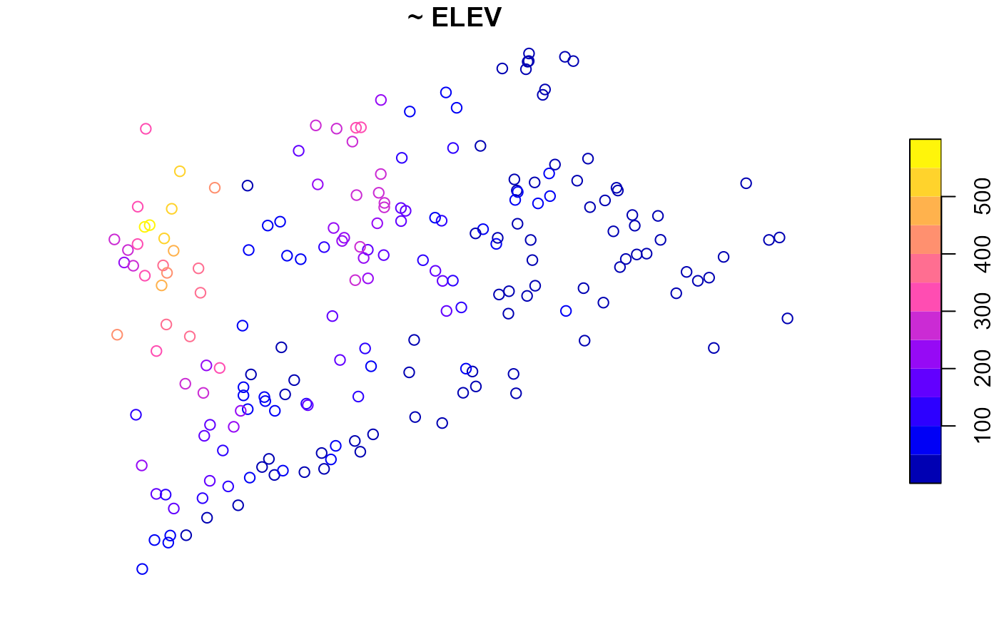
To summarize the distribution of ELEV_CAT, run
summary(NE_Lakes, formula = ~ ELEV_CAT)
#>    total     ELEV_CAT
#>  total:195   low :112
#>              high: 83
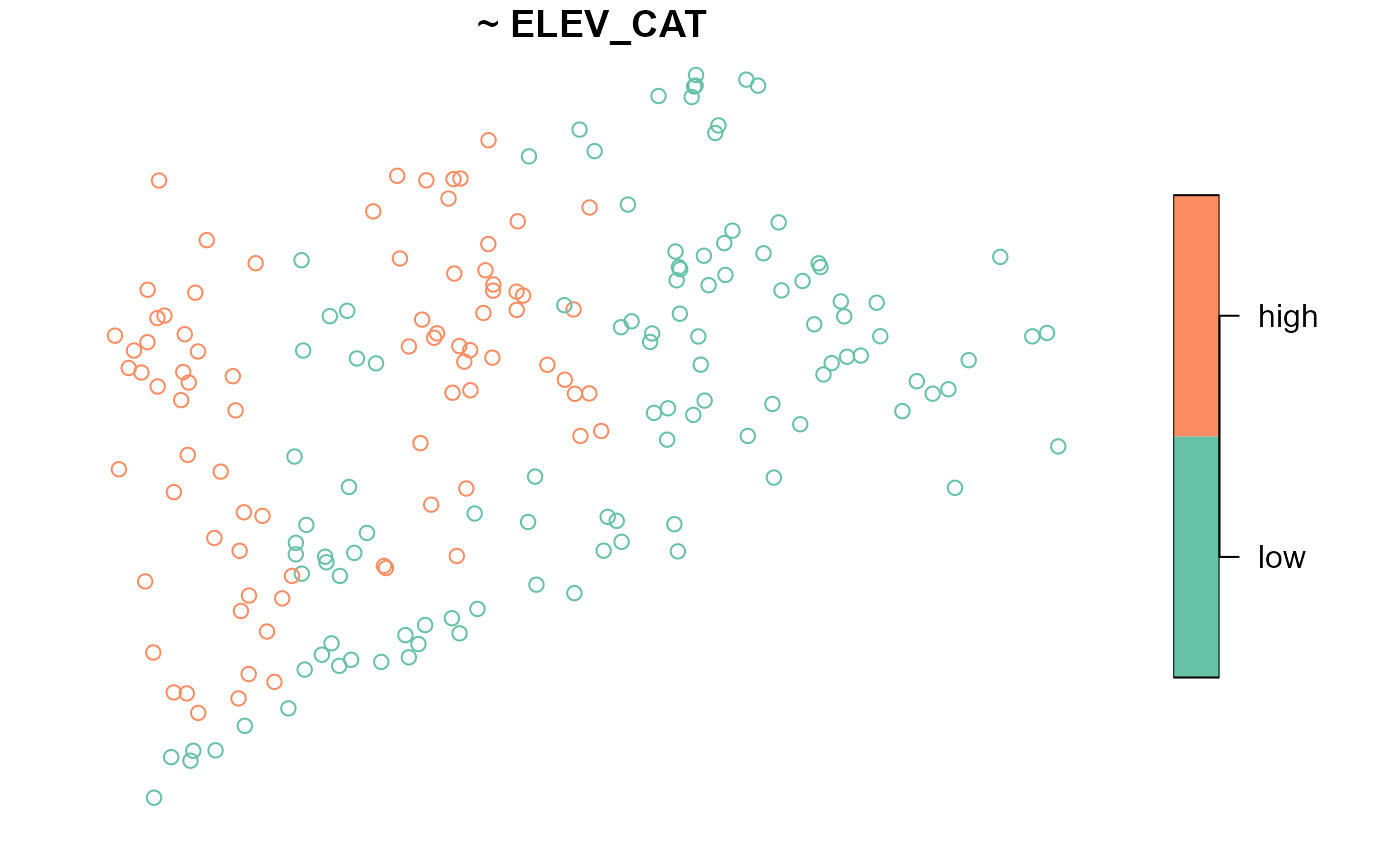
The ELEV_CAT column returns the number of lakes in each
elevation category. To visualize ELEV_CAT, run

The key.width argument extends the plot’s margin to fit
the legend text nicely within the plot. The plot’s default title is the
formula argument, though this is changed using the
main argument to plot().
The formula used by summary() and plot() is
quite flexible. Additional variables are included using
+:
summary(NE_Lakes, formula = ~ ELEV_CAT + AREA_CAT)
#>    total     ELEV_CAT    AREA_CAT
#>  total:195   low :112   small:135
#>              high: 83   large: 60
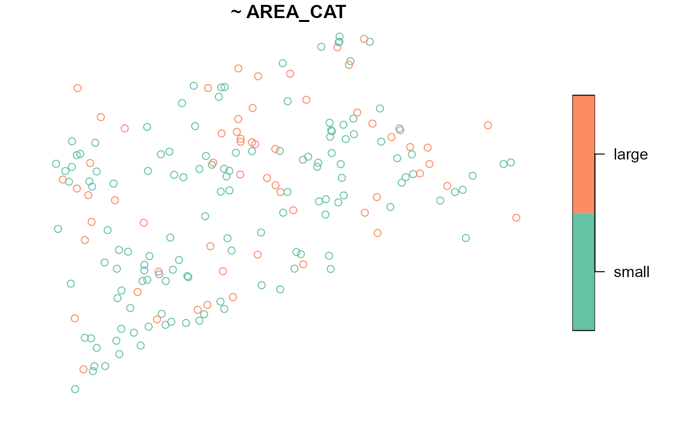
The plot() function returns two plots – one for
ELEV_CAT and another for AREA_CAT:
Interactions are included using the interaction operator,
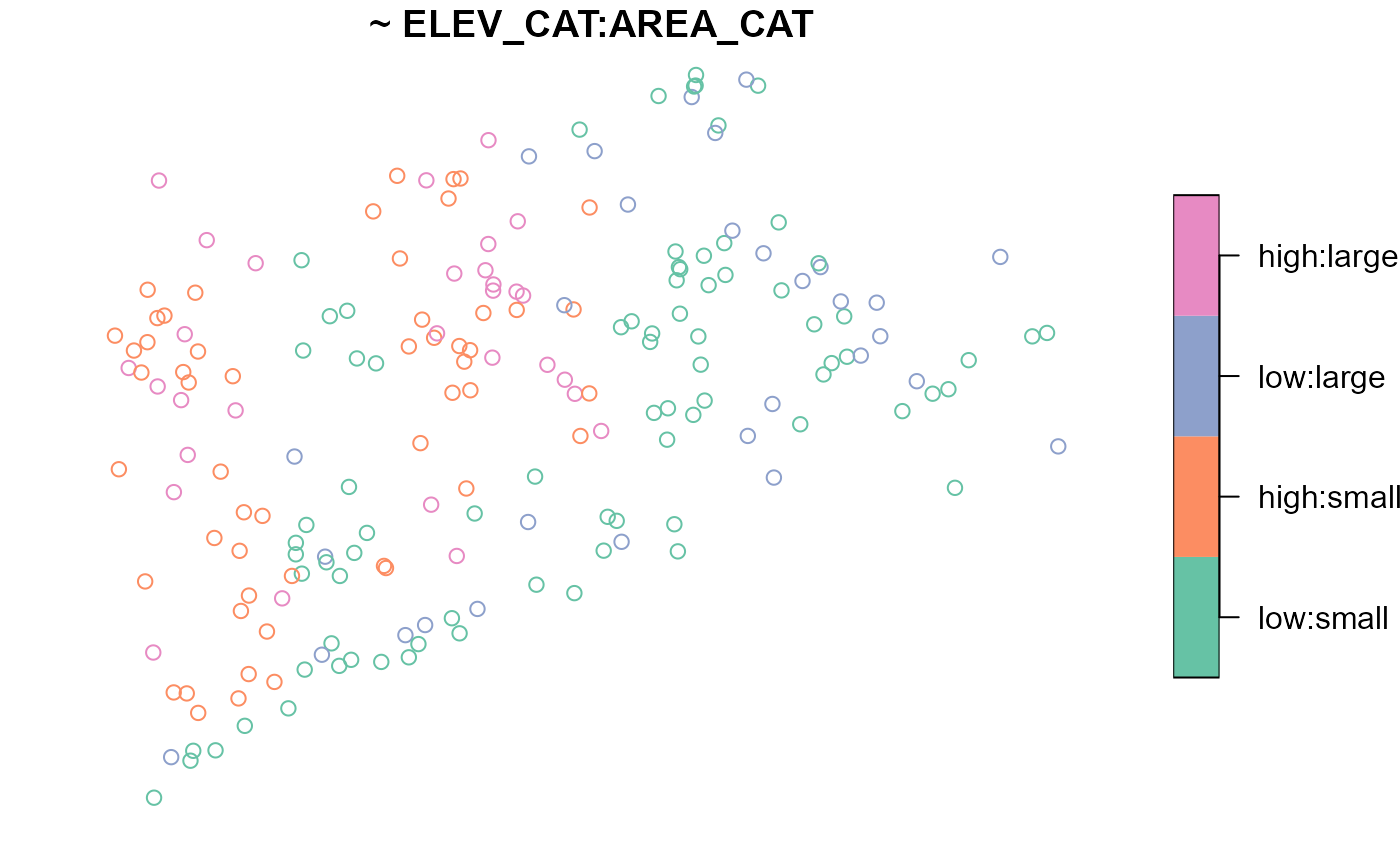
:. The interaction operator returns the interaction between
variables and is most useful when used with categorical variables. To
summarize the interaction between ELEV_CAT and
AREA_CAT, run
summary(NE_Lakes, formula = ~ ELEV_CAT:AREA_CAT)
#>    total      ELEV_CAT:AREA_CAT
#>  total:195   low:small :82
#>              high:small:53
#>              low:large :30
#>              high:large:30
Levels of each variable are separated by :. For example,
there are 86 lakes that are in the low elevation category and the small
area category. To visualize this interaction, run
The formula accommodates the * operator, which combines
the + and : operators. For example,
ELEV_CAT*AREA_CAT is shorthand for
ELEV_CAT + AREA_CAT + ELEV_CAT:AREA_CAT. The formula also
accommodates the . operator, which is shorthand for all
variables separated by +.
Two-sided formulas
Two-sided formulas are used to summarize the distribution of a
left-hand side variable for each level of each right-hand side variable.
To summarize the distribution of ELEV for each level of
AREA_CAT, run
summary(NE_Lakes, formula = ELEV ~ AREA_CAT)
#> ELEV by total:
#>       Min. 1st Qu. Median     Mean 3rd Qu.   Max.
#> total    0  21.925  69.09 127.3862 203.255 561.41
#>
#> ELEV by AREA_CAT:
#>       Min. 1st Qu.  Median     Mean  3rd Qu.   Max.
#> small 0.00   19.64  59.660 117.4473 176.1700 561.41
#> large 0.01   26.75 102.415 149.7487 241.2025 537.84
To visualize the distribution of ELEV for each level of
AREA_CAT, run
plot(NE_Lakes, formula = ELEV ~ AREA_CAT)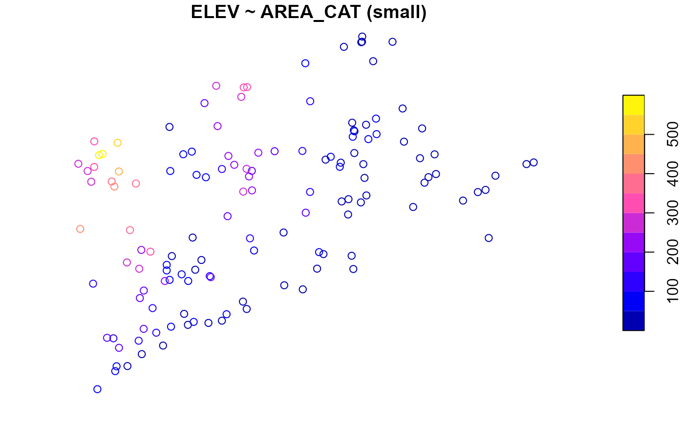
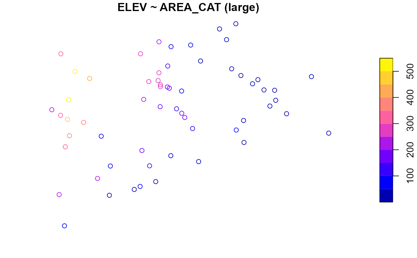
To only summarize or visualize a particular level of a single
right-hand side variable, use the onlyshow argument:
summary(NE_Lakes, formula = ELEV ~ AREA_CAT, onlyshow = "small")
#> ELEV by AREA_CAT:
#>       Min. 1st Qu. Median     Mean 3rd Qu.   Max.
#> small    0   19.64  59.66 117.4473  176.17 561.41
plot(NE_Lakes, formula = ELEV ~ AREA_CAT, onlyshow = "small")
To summarize the distribution of ELEV_CAT for each level
of AREA_CAT, run
summary(NE_Lakes, formula = ELEV_CAT ~ AREA_CAT)
#> ELEV_CAT by total:
#>       low high
#> total 112   83
#>
#> ELEV_CAT by AREA_CAT:
#>       low high
#> small  82   53
#> large  30   30
To visualize the distribution of ELEV_CAT for each level
of AREA_CAT, run

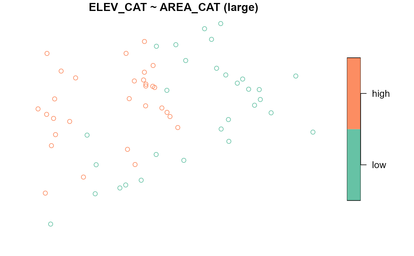
Adjusting graphical parameters
There are three arguments in plot() that can adjust
graphical parameters:
-
var_argsadjusts graphical parameters simultaneously for all levels of a variable -
varlevel_argsadjusts graphical parameters uniquely for each level of a variable -
...adjusts graphical parameters for simultaneously for all levels of all variables
The var_args and varlevel_args arguments
take lists whose names match variable names in the formula. For
varlevel_args, each list element must have an element named
levels that matches the variable’s levels. The following
example combines all three graphical parameter adjustment arguments:
list1 <- list(main = "Elevation Categories", pal = rainbow)
list2 <- list(main = "Area Categories")
list3 <- list(levels = c("small", "large"), pch = c(4, 19))
plot(
  NE_Lakes,
  formula = ~ ELEV_CAT + AREA_CAT,
  var_args = list(ELEV_CAT = list1, AREA_CAT = list2),
  varlevel_args = list(AREA_CAT = list3),
  cex = 0.75,
  key.width = lcm(3)
)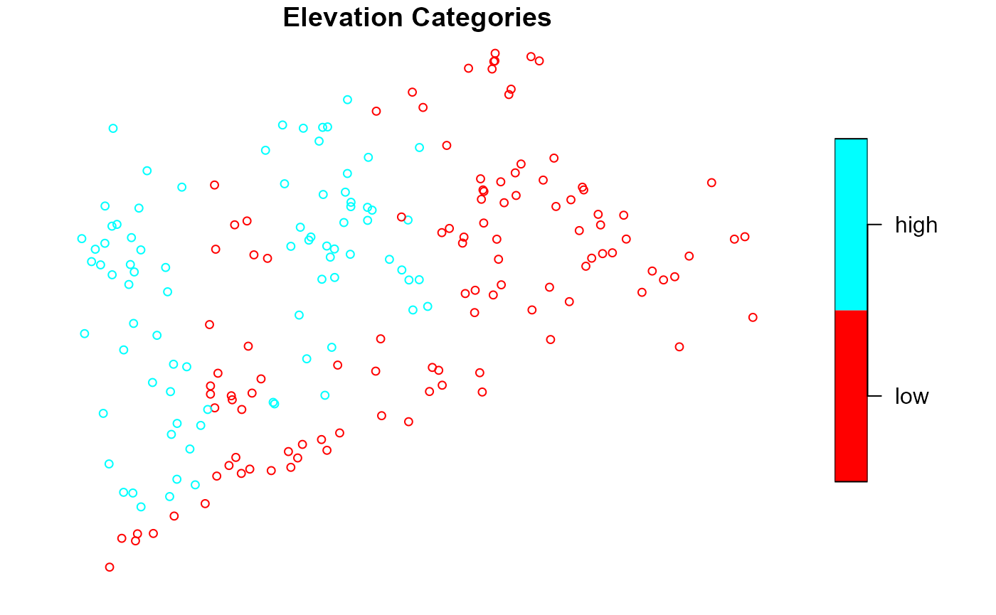
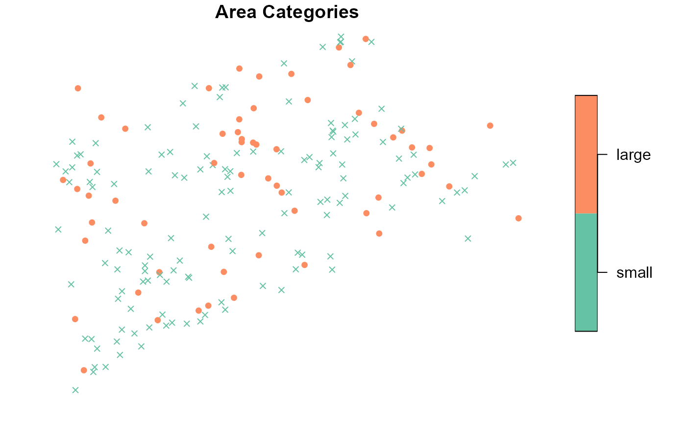
var_args uses list1 to give the
ELEV_CAT visualization a new title and color palette;
var_args uses list2 to give the
AREA_CAT visualization a new title;
varlevel_args uses list3 to give the
AREA_CAT visualization different shapes for the small and
large levels; ... uses cex = 0.75 to reduce
the size of all points; and ... uses key.width
to adjust legend spacing for all visualizations.
If a two-sided formula is used, it is possible to adjust graphical
parameters of the left-hand side variable for all levels of a right-hand
side variable. This occurs when a sublist matching the structure of
varlevel_args is used as an argument to
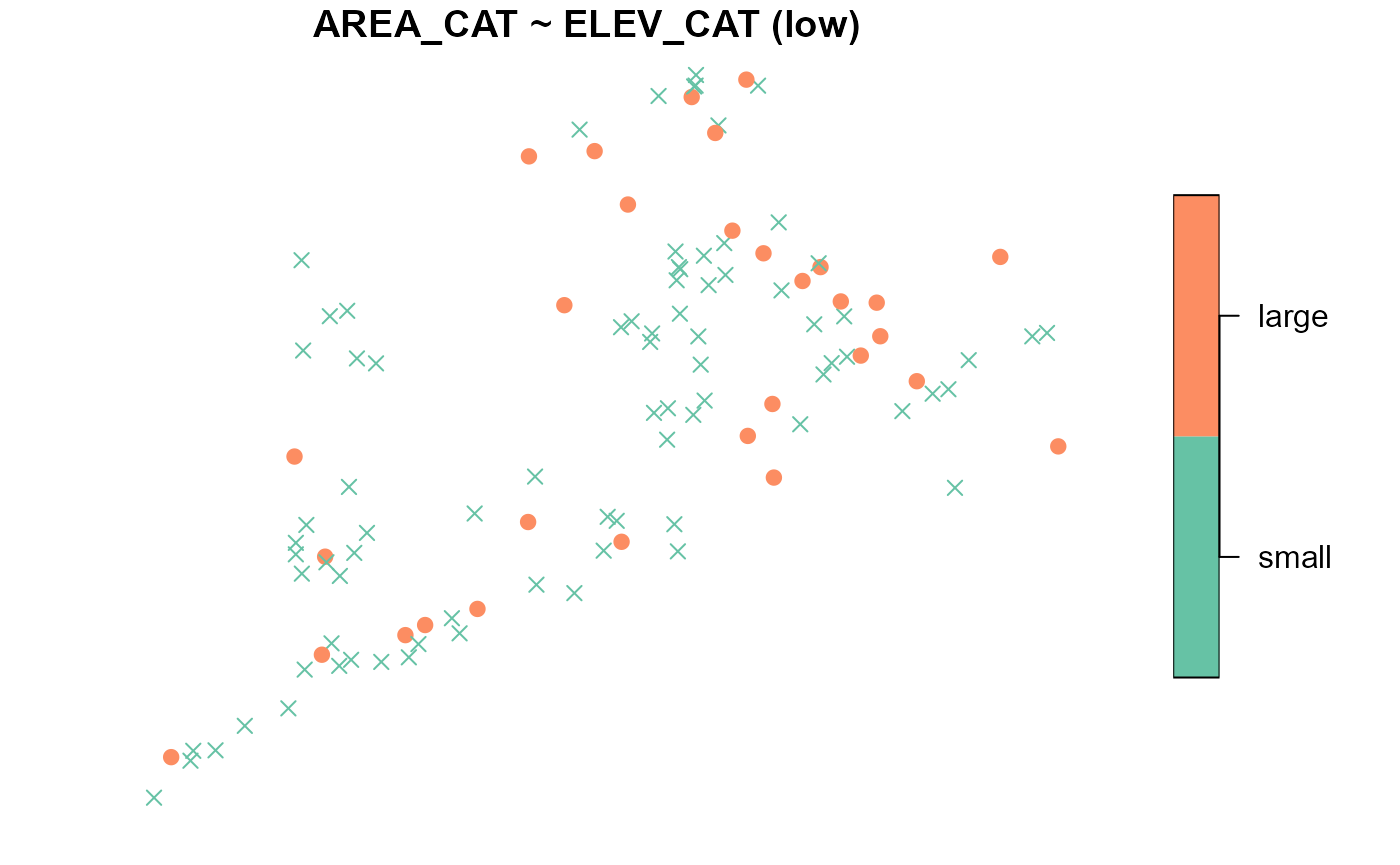
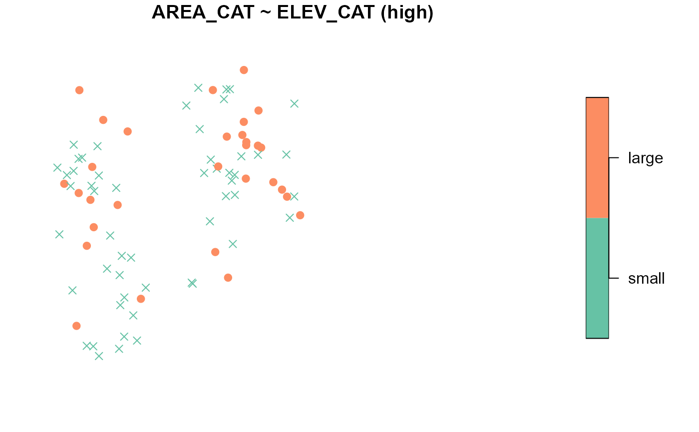
var_args. In this next example, different shapes are used
for the small and large levels of AREA_CAT for all levels
of ELEV_CAT:
sublist <- list(AREA_CAT = list3)
plot(
  NE_Lakes,
  formula = AREA_CAT ~ ELEV_CAT,
  var_args = list(ELEV_CAT = sublist),
  key.width = lcm(3)
)
Design sites
Design sites (output from the grts() or
irs() functions) can be summarized and visualized using
summary() and plot() very similarly to how
sampling frames were summarized and visualized in the previous section.
Soon you will use the grts() function to select a spatially
balanced sample. The grts() function does incorporate
randomness, so to match your results with this output exactly you will
need to set a reproducible seed by running
set.seed(51)First we will obtain some design sites: To select an equal probability GRTS sample of size 50 with 10 reverse hierarchically ordered replacement sites, run
eqprob_rho <- grts(NE_Lakes, n_base = 50, n_over = 10)Similar to summary() and plot() for
sampling frames, summary() and plot() for
design sites uses a formula. The formula should include
siteuse, which is the name of the variable in the design
sites object that indicates the type of each site. The default formula
for summary() and plot() is
~siteuse, which summarizes or visualizes the
sites objects in the design sites object. By default, the
formula is applied to all non-NULL sites
objects (in eqprob_rho, the nonNULL sites
objects are sites_base (for the base sites) and
sites_over (for the reverse hierarchically ordered
replacement sites)).
summary(eqprob_rho)
#>    total    siteuse
#>  total:60   Base:50
#>             Over:10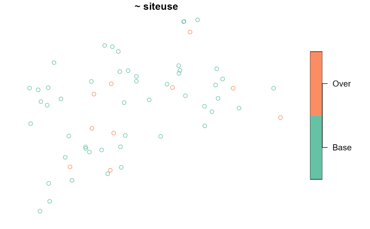
The sampling frame may be included as an argument to the
plot() function:
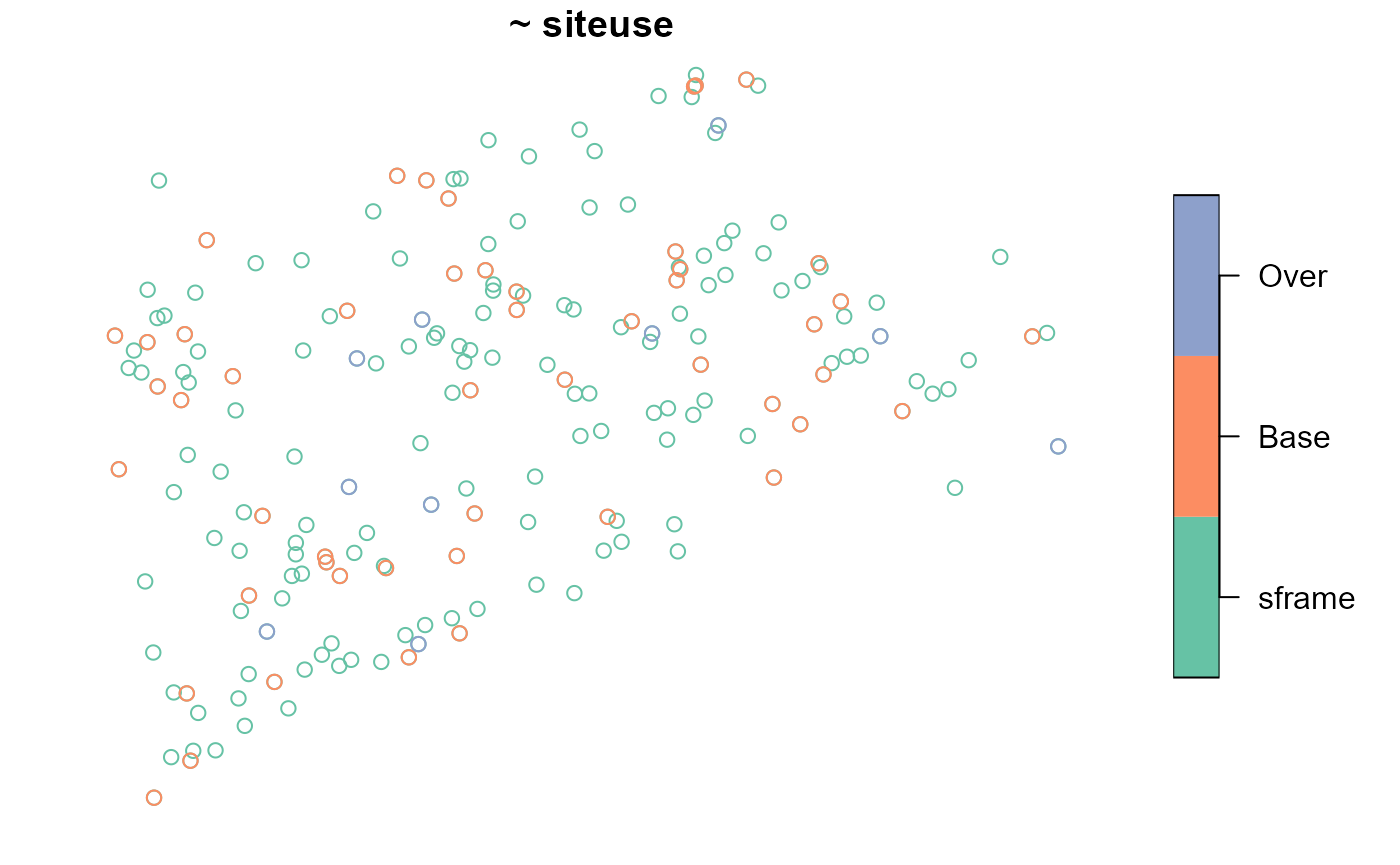
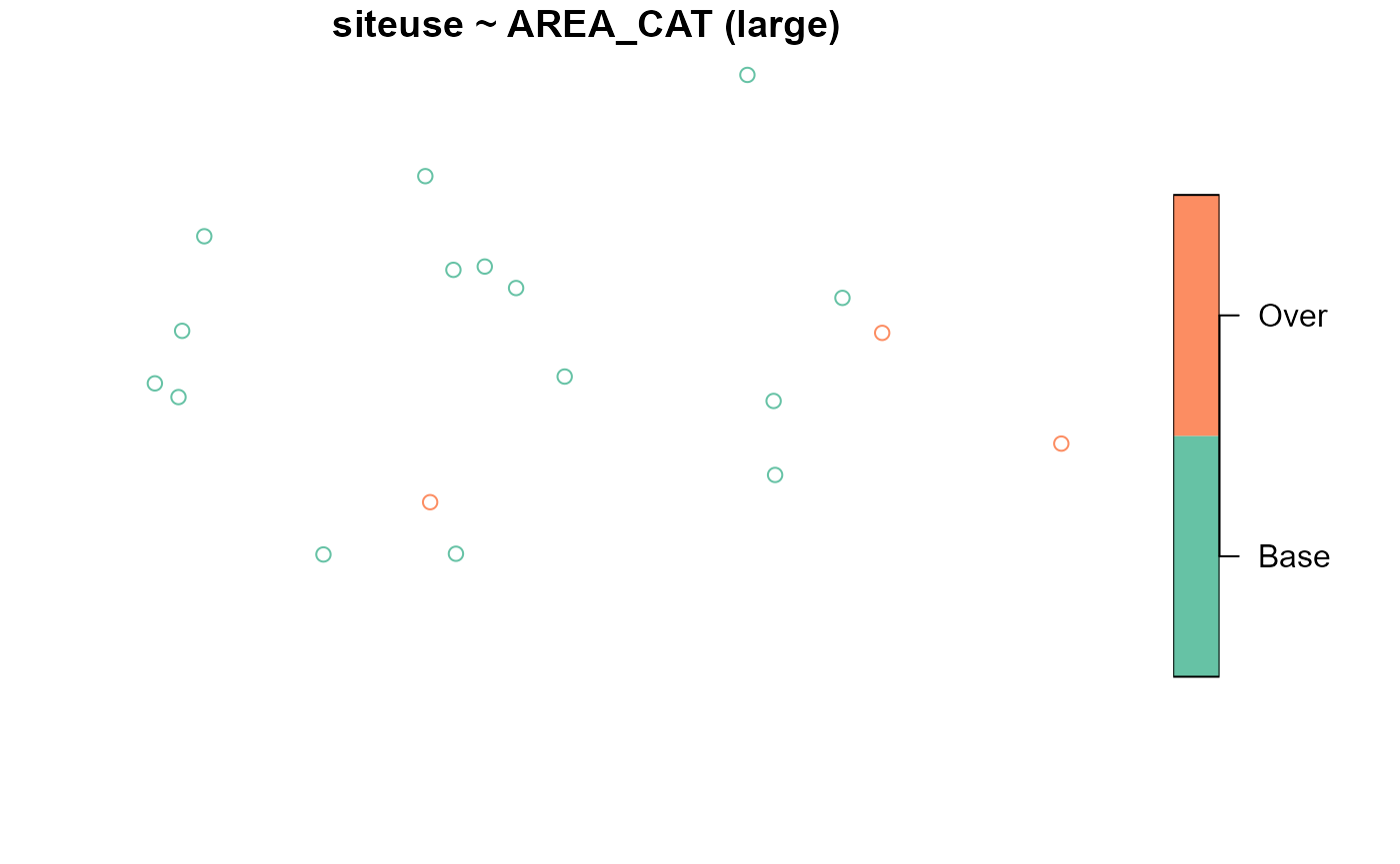
When you include siteuse as a left-hand side variable
(siteuse is treated as a categorical variable), you can
summarize and visualize the sites object for each level of
each right-hand side variable:
summary(eqprob_rho, formula = siteuse ~ AREA_CAT)
#> siteuse by total:
#>       Base Over
#> total   50   10
#>
#> siteuse by AREA_CAT:
#>       Base Over
#> small   35    7
#> large   15    3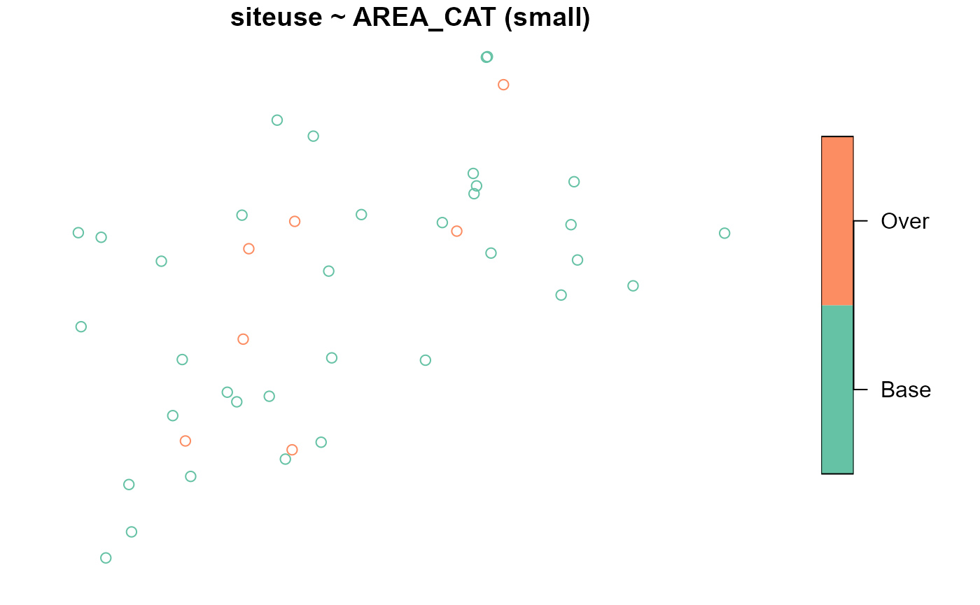
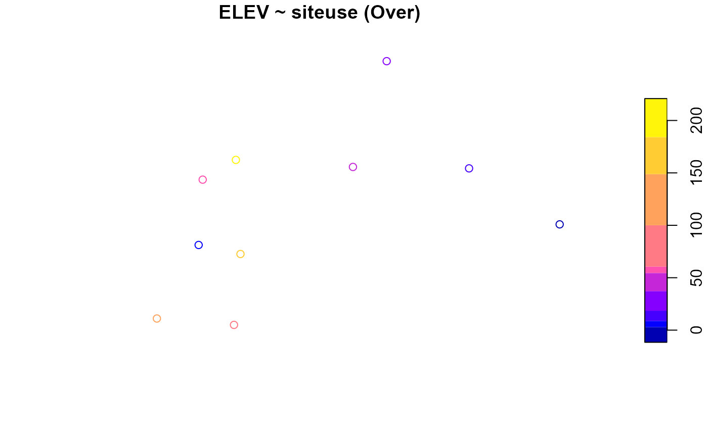
You can also summarize and visualize a left-hand side variable for
each level of siteuse:
summary(eqprob_rho, formula = ELEV ~ siteuse)
#> ELEV by total:
#>       Min. 1st Qu. Median    Mean  3rd Qu.   Max.
#> total 0.03  26.385 65.535 135.364 214.2075 537.84
#>
#> ELEV by siteuse:
#>      Min. 1st Qu. Median     Mean 3rd Qu.   Max.
#> Base 0.68 29.4850  81.76 148.0362 263.640 537.84
#> Over 0.03 15.1275  54.49  72.0030 119.365 209.25
plot(eqprob_rho, formula = ELEV ~ siteuse)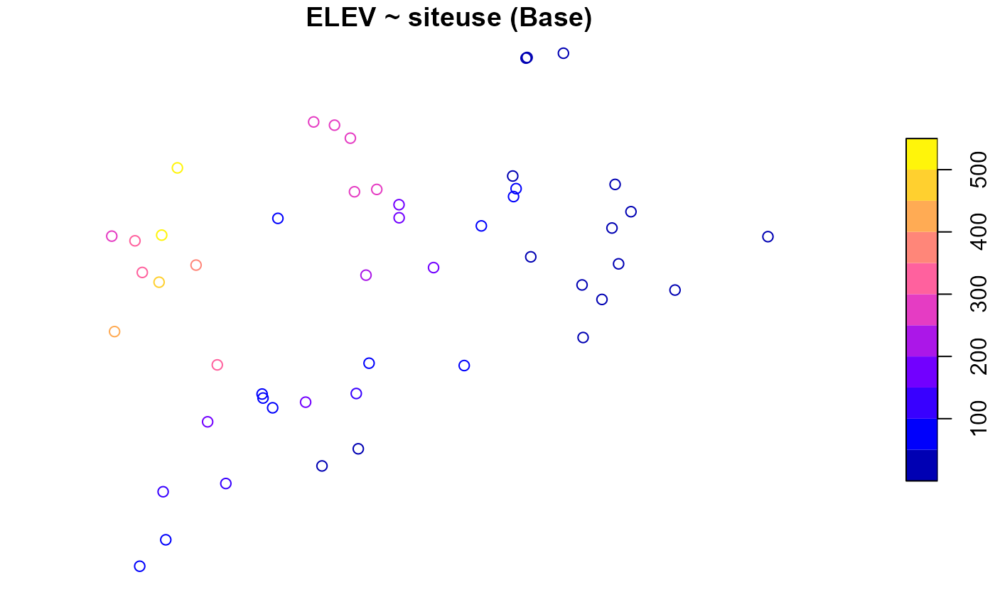
Analysis data
sp_summarize() and plot() work for analysis
data the same way they do for sampling frames. The NLA_PNW
analysis data in spsurvey is analysis data (as an sf
object) from lakes in California, Oregon, and Washington. There are two
variables in NLA_PNW you will use next:
-
STATE: state name (California,Washington, andOregon) -
NITR_COND: nitrogen content categories (Poor,Fair, andGood)
Before summarizing or visualizing a sampling frame, turn it into an
object using sp_frame():
NLA_PNW <- sp_frame(NLA_PNW)To summarize and visualize NITR_COND across all states,
run
summary(NLA_PNW, formula = ~ NITR_COND)
#>    total    NITR_COND
#>  total:96   Fair:24
#>             Good:38
#>             Poor:34
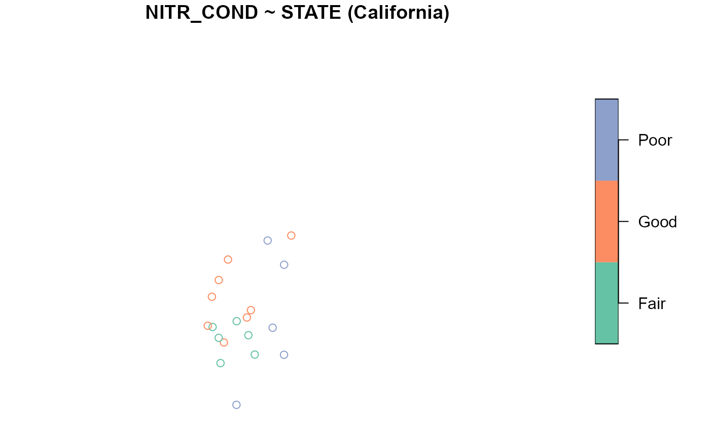
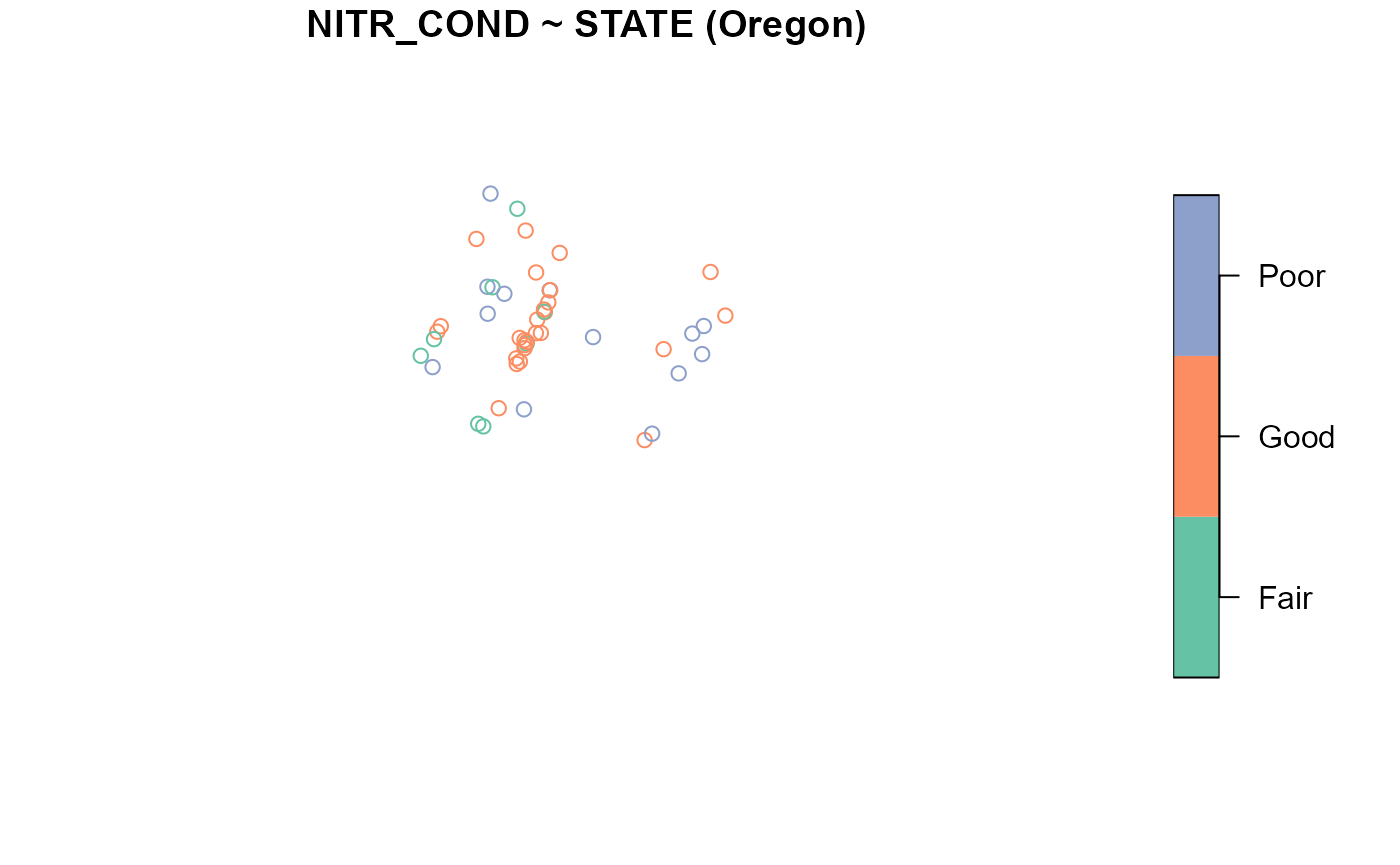
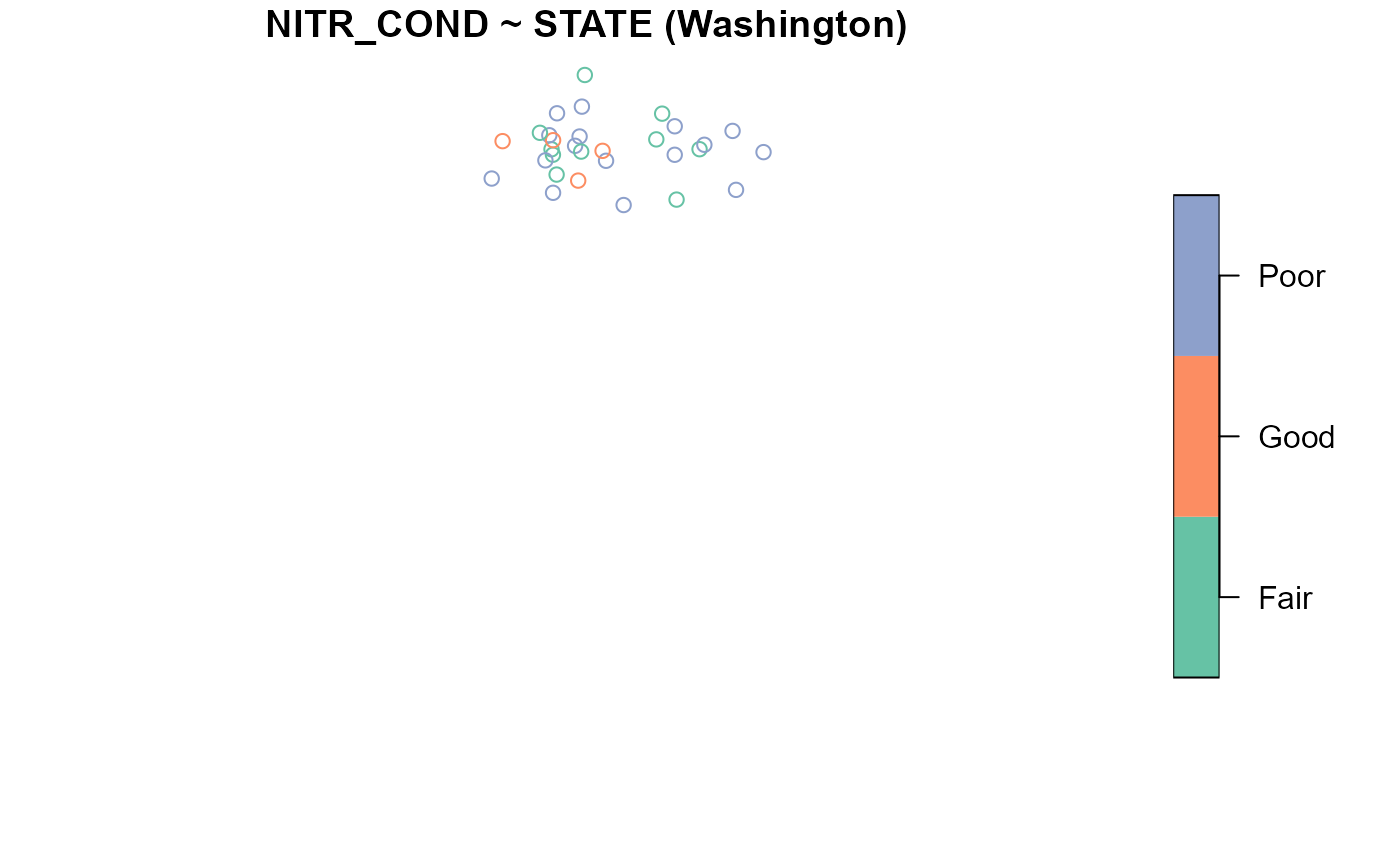
Suppose the sampling design was stratified by STATE. To
summarize and visualize NITR_COND by STATE,
run
summary(NLA_PNW, formula = NITR_COND ~ STATE)
#> NITR_COND by total:
#>       Fair Good Poor
#> total   24   38   34
#>
#> NITR_COND by STATE:
#>            Fair Good Poor
#> California    6    8    5
#> Oregon        8   26   13
#> Washington   10    4   16