(9) A Physiologically Based Pharmacokinetic Model

Dustin Kapraun

2025-09-01

Model Description

Like any pharmacokinetic (PK) model, a physiologically based pharmacokinetic (PBPK) model is a mathematical description of the absorption, distribution, metabolism, and excretion of a substance by an organism. PBPK models differ from classical PK models in that many of their parameters describe actual anatomical and physiological properties of the organism, such as volumes of and blood flow rates to various organs and tissues. Figure 1 shows a schematic representation of a relatively simple PBPK model for “Substance X.”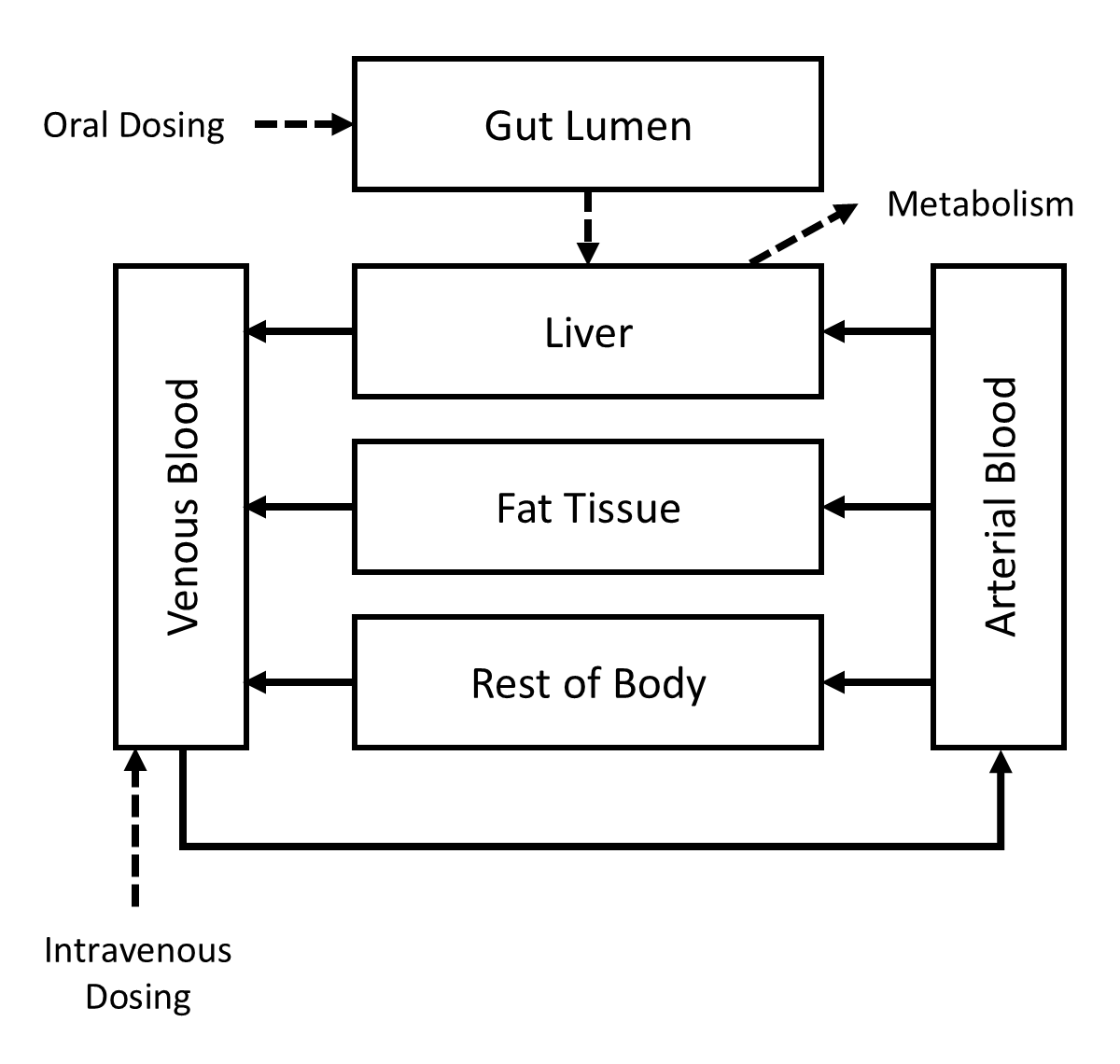

Figure 1: A simple PBPK model

Substance X can enter the body through oral and/or intravenous routes and it is eliminated via saturable metabolism in the liver. The kinetics of distribution are assumed to be “perfusion limited,” so concentrations in different tissues depend on steady state concentration ratios, or “partition coefficients,” for each type of tissue.

The state variables for the PBPK model include:

• $A_\textrm{G}$, the amount (of Substance X) in the gut lumen (mg);
• $A_\textrm{L}$, the amount in the liver (mg);
• $A_\textrm{F}$, the amount in the fat (mg);
• $A_\textrm{AB}$, the amount in the arterial blood (mg);
• $A_\textrm{VB}$, the amount in the venous blood (mg);
• $A_\textrm{R}$, the amount in the rest of body (mg);
• $A_\textrm{dose}$, the cumulative amount that has been dosed (mg); and
• $A_\textrm{m}$, the cumulative amount that has been metabolized (mg).

The anatomical and physiological parameters are:

• $M$, the body mass of the organism (kg);
• $Q_\textrm{CC}$, the cardiac output constant (L/h/kg${}^{0.75}$, i.e., liters per hour per kg of body mass to the 3/4 power);
• $Q_\textrm{LC}$, the constant fractional blood flow to the liver;
• $Q_\textrm{FC}$, the constant fractional blood flow to the fat;
• $V_\textrm{LC}$, the constant volume fraction of body mass that is the liver (L/kg);
• $V_\textrm{FC}$, the constant volume fraction of body mass that is the fat (L/kg);
• $V_\textrm{ABC}$, the constant volume fraction of body mass that is the arterial blood (L/kg); and
• $V_\textrm{VBC}$, the constant volume fraction of body mass that is the venous blood (L/kg).

Values for anatomical and physiological parameters for rats and humans are shown in the following table.

Parameter	Units	Rat Value	Human Value
$M$	kg	0.25	80
$Q_\textrm{CC}$	L/h/kg${}^{0.75}$	15	15
$Q_\textrm{LC}$	–	0.21	0.26
$Q_\textrm{FC}$	–	0.06	0.05
$V_\textrm{LC}$	L/kg	0.04	0.02
$V_\textrm{FC}$	L/kg	0.07	0.21
$V_\textrm{ABC}$	L/kg	0.02	0.02
$V_\textrm{VBC}$	L/kg	0.05	0.05

The chemical-specific parameters for Substance X are:

• $P_\textrm{L} = 3.5$, the liver-to-blood partition coefficient;
• $P_\textrm{F} = 86.5$, the fat-to-blood partition coefficient;
• $P_\textrm{R} = 2.3$, the rest-of-body-to-blood partition coefficient;
• $V_\textrm{maxC} = 10.0$, the maximum metabolic rate constant (mg/h/kg${}^{0.75}$);
• $K_\textrm{m} = 6.0$, the affinity constant for saturable metabolism (mg/L); and
• $k_\textrm{abs} = 1.25$, the first-order oral absorption rate constant (h${}^{-1}$).

In general, chemical-specific parameters can have different values for different animal species but, in this case, we assume that they have the same values for rats and humans.

The dosing parameters are:

• $D_\textrm{oral}$, the body mass normalized daily oral dose rate (mg/kg/d); and
• $D_\textrm{IV}$, the body mass normalized daily intravenous dose rate (mg/kg/d).

Note that the dosing rates are given in units of mg of Substance X per kg of body mass per day.

To construct the state equations for the model, the following “calculated parameters” are needed:

• $Q_\textrm{C} = Q_\textrm{CC} \cdot M^{0.75}$, cardiac output (L/h);
• $Q_\textrm{L} = Q_\textrm{LC} \cdot Q_\textrm{C}$, blood flow rate to the liver (L/h);
• $Q_\textrm{F} = Q_\textrm{FC} \cdot Q_\textrm{C}$, blood flow rate to the fat (L/h);
• $Q_\textrm{RC} = 1.0 - (Q_\textrm{LC} + Q_\textrm{FC})$, constant fractional blood flow to the rest of body;
• $Q_\textrm{R} = Q_\textrm{RC} \cdot Q_\textrm{C}$, blood flow rate to the rest of body (L/h);
• $V_\textrm{L} = V_\textrm{LC} \cdot M$, volume of the liver (L);
• $V_\textrm{F} = V_\textrm{FC} \cdot M$, volume of the fat (L);
• $V_\textrm{AB} = V_\textrm{ABC} \cdot M$, volume of the arterial blood (L);
• $V_\textrm{VB} = V_\textrm{VBC} \cdot M$, volume of the venous blood (L);
• $V_\textrm{RC} = 1.0 - (V_\textrm{LC} + V_\textrm{FC} + V_\textrm{ABC} + V_\textrm{VBC})$, constant volume fraction of body mass that is the rest of body (L/kg);
• $V_\textrm{R} = V_\textrm{RC} \cdot M$, volume of the rest of body (L);
• $V_\textrm{max} = V_\textrm{maxC} \cdot M^{0.75}$, maximum rate of metabolism (mg/h);
• $R_\textrm{oral} = D_\textrm{oral} \cdot M / 24$, the oral dose rate (mg/h); and
• $R_\textrm{IV} = D_\textrm{IV} \cdot M / 24$, the intravenous dose rate (mg/h);

In addition to the model parameters, the following time-varying quantities are needed to construct the state equations:

• $C_\textrm{L}(t) = \frac{A_\textrm{L}(t)}{V_\textrm{L}}$, the concentration (of Substance X) in the liver (mg/L) at time $t$;
• $C_\textrm{F}(t) = \frac{A_\textrm{F}(t)}{V_\textrm{F}}$, the concentration in the fat (mg/L) at time $t$;
• $C_\textrm{AB}(t) = \frac{A_\textrm{AB}(t)}{V_\textrm{AB}}$, the concentration in the arterial blood (mg/L) at time $t$;
• $C_\textrm{VB}(t) = \frac{A_\textrm{VB}(t)}{V_\textrm{VB}}$, the concentration in the venous blood (mg/L) at time $t$;
• $C_\textrm{R}(t) = \frac{A_\textrm{R}(t)}{V_\textrm{R}}$, the concentration in the rest of body (mg/L) at time $t$;
• $R_\textrm{m}(t) = \frac{V_\textrm{max} \cdot C_\textrm{L}(t) / P_\textrm{L}}{ K_\textrm{m} + C_\textrm{L}(t) / P_\textrm{L}}$, the rate of metabolism in the liver (mg/h) at time $t$; and
• $R_\textrm{abs}(t) = k_\textrm{abs} \cdot A_\textrm{G}(t)$, the rate of absorption from the gut lumen to the liver (mg/h) at time $t$.

The state equations for the PBPK model are:

• $\frac{\textrm{d}}{\textrm{d}t} A_\textrm{G}(t) = R_\textrm{oral} - R_\textrm{abs}(t)$;
• $\frac{\textrm{d}}{\textrm{d}t} A_\textrm{L}(t) = Q_\textrm{L} \cdot \left( C_\textrm{AB}(t) - \frac{C_\textrm{L}(t)}{P_\textrm{L}} \right) + R_\textrm{abs}(t) - R_\textrm{m}(t)$;
• $\frac{\textrm{d}}{\textrm{d}t} A_\textrm{F}(t) = Q_\textrm{F} \cdot \left( C_\textrm{AB}(t) - \frac{C_\textrm{F}(t)}{P_\textrm{F}} \right)$;
• $\frac{\textrm{d}}{\textrm{d}t} A_\textrm{AB}(t) = Q_\textrm{C} \cdot \left( C_\textrm{VB}(t) - C_\textrm{AB}(t) \right)$;
• $\frac{\textrm{d}}{\textrm{d}t} A_\textrm{VB}(t) = Q_\textrm{L} \cdot \frac{C_\textrm{L}(t)}{P_\textrm{L}} + Q_\textrm{F} \cdot \frac{C_\textrm{F}(t)}{P_\textrm{F}} + Q_\textrm{R} \cdot \frac{C_\textrm{R}(t)}{P_\textrm{R}} - Q_\textrm{C} \cdot C_\textrm{VB}(t) + R_\textrm{IV}$;
• $\frac{\textrm{d}}{\textrm{d}t} A_\textrm{R}(t) = Q_\textrm{R} \cdot \left( C_\textrm{AB}(t) - \frac{C_\textrm{R}(t)}{P_\textrm{R}} \right)$;
• $\frac{\textrm{d}}{\textrm{d}t} A_\textrm{dose}(t) = R_\textrm{oral} + R_\textrm{IV}$; and
• $\frac{\textrm{d}}{\textrm{d}t} A_\textrm{m}(t) = R_\textrm{m}(t)$.

In order to solve an initial value problem for the PBPK model, one needs to provide the values of the basic parameters (but not the calculated parameters) and initial values for all the state variables.

MCSim Model Specification

We used the GNU MCSim model specification language to implement the simple PBPK model for Substance X. The complete MCSim model specification file for this model, pbpk_simple.model, can be found in the extdata subdirectory of the MCSimMod package installation directory.

In addition to the state variables that have already been described, we included a state variable that represents the area under the venous blood concentration vs. time curve (AUC), as this is a quantity that is often computed in pharmacokinetic analyses. The AUC for the period from time $0$ to time $t$ is given by $\textrm{AUC}(t) = \int_0^t C_\textrm{VB}(\tau) \, \textrm{d}\tau$ and thus the state equation for this quantity is $$\begin{equation} \frac{\textrm{d}}{\textrm{d}t} \textrm{AUC}(t) = C_\textrm{VB}(t). \end{equation}$$

Also, in addition to the time-varying quantities previously mentioned, the model includes another output variable, $$\begin{equation} A_\textrm{tot}(t) = A_\textrm{dose}(t) - \left( A_\textrm{G}(t) + A_\textrm{F}(t) + A_\textrm{AB}(t) + A_\textrm{VB}(t) + A_\textrm{R}(t) \right) - A_\textrm{m}(t), \end{equation}$$ that represents the total amount of substance that has been “lost” vs. time. This amount is calculated as [total (cumulative) amount that has entered in the organism] - [total amount currently in the organism] - [total (cumulative) amount that has been eliminated from the organism]. Therefore, if the model “conserves mass” as it should, the value of $A_\textrm{tot}(t)$ should be zero (or very close to zero for numerical solutions to an IVP) at all times $t$.

Note that the model specification file uses text symbols to represent the state variables, output variables, and parameters in the model. For example, the state variable $A_\textrm{L}$ is represented by the text symbol A_L, the output variable $C_\textrm{L}$ is represented by the text symbol C_L, and the parameter $Q_\textrm{LC}$ is represented by the text symbol Q_LC.

Building the Model

First, we load the MCSimMod package as follows.

library(MCSimMod)

Using the following commands, we create a model object (i.e., an instance of the Model class) using the model specification file pbpk_simple.model that is included in the MCSimMod package.

# Get the full name of the package directory that contains the example MCSim
# model specification file.
mod_path <- file.path(system.file(package = "MCSimMod"), "extdata")

# Create a model object using the example MCSim model specification file
# "pbpk_simple.model" included in the MCSimMod package.
pbpk_mod_name <- file.path(mod_path, "pbpk_simple")
pbpk_mod <- createModel(pbpk_mod_name)

This last command creates a Model object called pbpk_mod. Once that object is created, we can “load” the model (so that it’s ready for use in a given R session) as follows.

# Load the model.
pbpk_mod$loadModel()

Verifying Conservation of Mass

We can demonstrate that the PBPK model for Substance X conserves mass by performing a simulation in which a rat is orally administered 1 mg/kg/d of Substance X and plotting total amount of substance lost, $A_\textrm{tot}(t)$, vs. time, $t$.

The default values of the anatomical and physiological model parameters that are provided in the model specification file, pbpk_simple.model, are for a rat, and these are the values that are assigned to the parameters when one calls the loadModel() method. This can be verified by examining the attribute parms of the Model object pbpk_mod as follows.

pbpk_mod$parms
#>          M       Q_CC       Q_LC       Q_FC       V_LC       V_FC      V_ABC
#>  0.2500000 15.0000000  0.2100000  0.0600000  0.0400000  0.0700000  0.0200000
#>      V_VBC        P_L        P_F        P_R     V_maxC        K_m      k_abs
#>  0.0500000  3.5000000 86.5000000  2.3000000 10.0000000  6.0000000  1.2500000
#>     D_oral       D_IV        Q_C        Q_L        Q_F       Q_RC        Q_R
#>  0.0000000  0.0000000  5.3033009  1.1136932  0.3181981  0.7300000  3.8714096
#>        V_L        V_F       V_AB       V_VB       V_RC        V_R      V_max
#>  0.0100000  0.0175000  0.0050000  0.0125000  0.8200000  0.2050000  3.5355339
#>     R_oral       R_IV
#>  0.0000000  0.0000000

We want to perform a simulation in which a rat is orally administered 1 mg/kg/d of Substance X, so we will change the value of the parameter $D_\textrm{oral}$ from 0 to 1.

pbpk_mod$updateParms(c(D_oral = 1))

Now, if we examine the values of the model parameters, we can see that the body mass normalized oral administration rate (represented by $D_\textrm{oral}$ and D_oral) has been updated from 0 to 1 mg/kg/d and the actual oral administration rate (represented by (represented by $R_\textrm{oral}$ and R_oral), which is a calculated parameter, has also been updated (from 0 to approximately 0.0104 mg/h).

pbpk_mod$parms
#>           M        Q_CC        Q_LC        Q_FC        V_LC        V_FC
#>  0.25000000 15.00000000  0.21000000  0.06000000  0.04000000  0.07000000
#>       V_ABC       V_VBC         P_L         P_F         P_R      V_maxC
#>  0.02000000  0.05000000  3.50000000 86.50000000  2.30000000 10.00000000
#>         K_m       k_abs      D_oral        D_IV         Q_C         Q_L
#>  6.00000000  1.25000000  1.00000000  0.00000000  5.30330086  1.11369318
#>         Q_F        Q_RC         Q_R         V_L         V_F        V_AB
#>  0.31819805  0.73000000  3.87140963  0.01000000  0.01750000  0.00500000
#>        V_VB        V_RC         V_R       V_max      R_oral        R_IV
#>  0.01250000  0.82000000  0.20500000  3.53553391  0.01041667  0.00000000

We can examine the initial conditions for the state variables in the model using the following command.

pbpk_mod$Y0
#>    A_G    A_L    A_F   A_AB   A_VB    A_R A_dose    A_m    AUC
#>      0      0      0      0      0      0      0      0      0

As stated in the model specification file, pbpk_simple.model, the default values for the initial conditions are all zero.

Suppose that we want to perform a simulation and generate results for 100 hours following oral administration with an output resolution of 0.1 hours. We can create a vector of desired output times (i.e., $t = 0, 0.1, 0.2, \ldots, 100.0$) using the following command.

times <- seq(from = 0, to = 100, by = 0.1)

Then, we can perform the simulation and store the results in a “matrix” data structure called out_oral as follows.

out_oral <- pbpk_mod$runModel(times)

Finally, we can plot the total amount lost vs. time using the following command.

plot(out_oral[, "time"], out_oral[, "A_tot"],
  type = "l", lty = 1, lwd = 2,
  xlab = "Time (h)", ylab = "Amount (mg)"
)

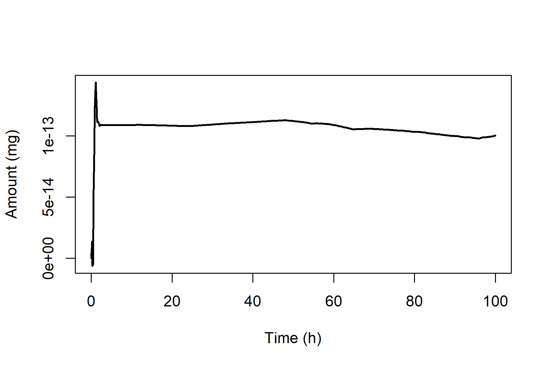Note that the total amount lost is close to zero (less than 10${}^{-12}$) at all time points examined. The degree of “closeness” to zero is determined by the numerical precision of the ODE solver, which can be adjusted using the arguments rtol and atol passed through runModel() to the deSolve function ode. Further details about these arguments can be found the documentation for the deSolve package.

Verifying Conservation of Flow

We can also verify that the total blood flow to the non-blood compartments in our PBPK model equals the total cardiac output using the following commands.

cat(
  "Total blood flow to compartments:",
  pbpk_mod$parms[["Q_L"]] + pbpk_mod$parms[["Q_F"]] + pbpk_mod$parms[["Q_R"]],
  "L/h\n"
)
#> Total blood flow to compartments: 5.303301 L/h
cat("Total cardiac output:", pbpk_mod$parms[["Q_C"]], "L/h\n")
#> Total cardiac output: 5.303301 L/h

Examining the Simulation Results

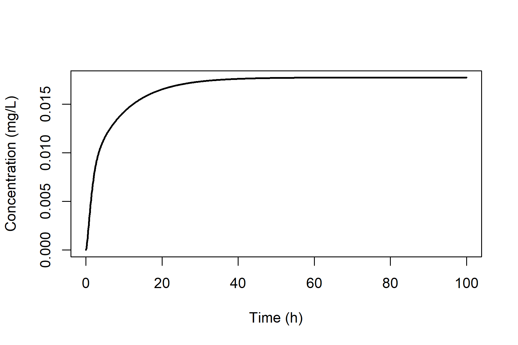
After performing a simulation and storing the results (in this case, in out_oral), we can create visual representations of these results. For example, we can plot the venous blood concentration vs. time using the following commands.

plot(out_oral[, "time"], out_oral[, "C_VB"],
  type = "l", lty = 1, lwd = 2,
  xlab = "Time (h)", ylab = "Concentration (mg/L)"
)

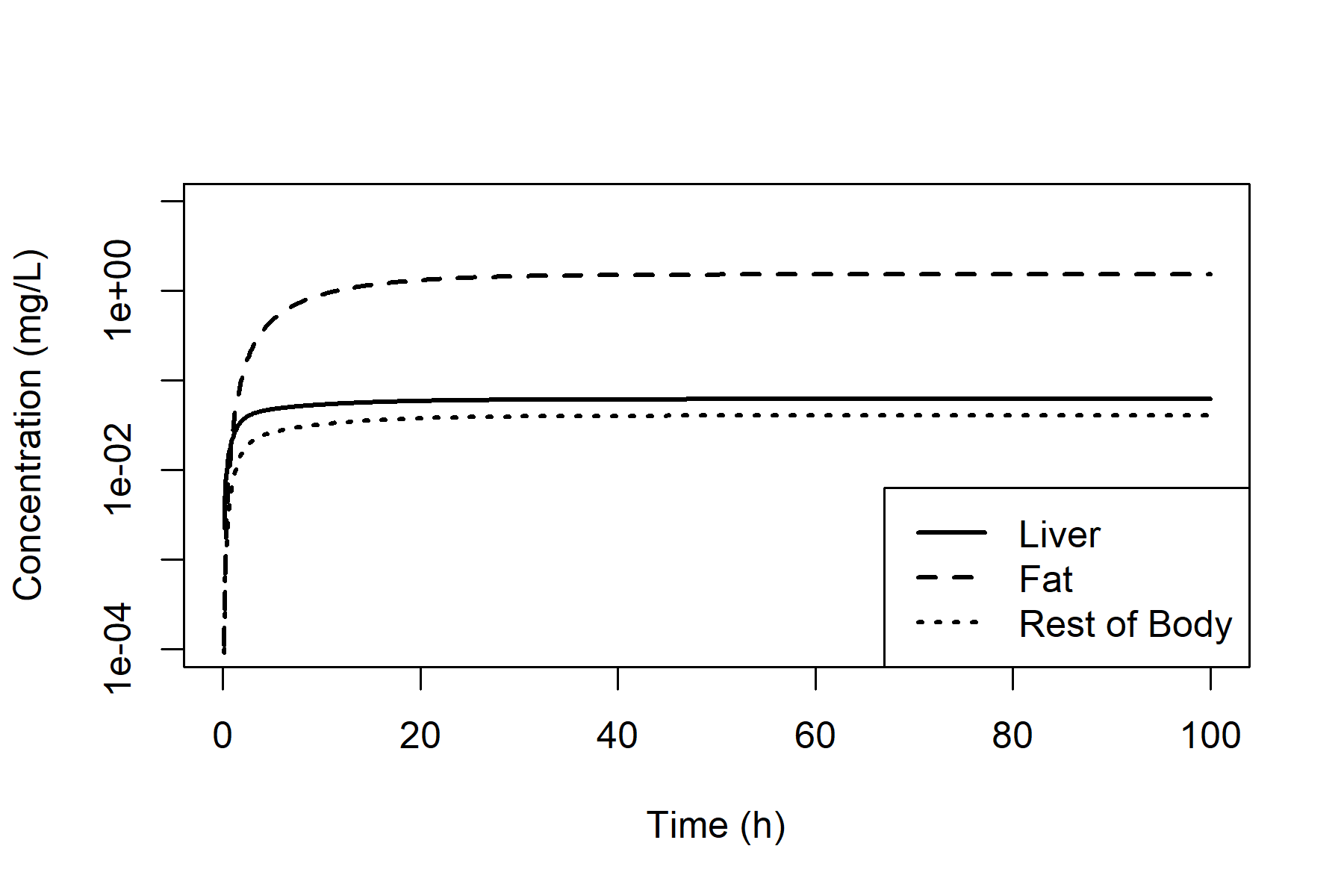
We can plot the concentrations in all non-blood compartments (on a logarithmic scale) as follows.

plot(out_oral[, "time"], out_oral[, "C_L"],
  type = "l", lty = 1, lwd = 2,
  log = "y", ylim = c(0.0001, 10),
  xlab = "Time (h)", ylab = "Concentration (mg/L)"
)
lines(out_oral[, "time"], out_oral[, "C_F"],
  lty = 2, lwd = 2
)
lines(out_oral[, "time"], out_oral[, "C_R"],
  lty = 3, lwd = 2
)
legend("bottomright",
  legend = c("Liver", "Fat", "Rest of Body"),
  lty = c(1, 2, 3), lwd = 2
)