The package nsink implements an approach to estimate
relative nitrogen removal along a flow path. This approach is detailed
in Kellogg et al. (2010) and builds on
peer-reviewed literature in the form of reviews and meta-analyses (Seitzinger et al. 2006, Alexander et al. 2007, i.e.,
Mayer et al. 2007) to estimate nitrogen (N) removal within three
types of landscape sinks – wetlands, streams and lakes – along any given
flow path within a HUC12 basin. The nsink package
implements this approach, using publicly available spatial data to
identify flow paths and estimate N removal in landscape sinks. Removal
rates depend on retention time, which is influenced by physical
characteristics identified using publicly available spatial data –
National Hydrography Dataset Plus (NHDPlus), Soil Survey Geographic
Database (SSURGO), the National Land Cover Dataset (NLCD) land cover,
and the National Land Cover Dataset (NLCD) impervious surface. Static
maps of a specified HUC-12 basin are generated – N Removal Efficiency, N
Loading Index, N Transport Index, and N Delivery Index. These maps may
be used to inform local decision-making by highlighting areas that are
more prone to N “leakiness” and areas that contribute to N removal.
The nsink package provides several functions to set up
and run an N-Sink analysis for a specified 12-digit HUC code. All
required data are downloaded, prepared for the analysis, HUC-wide
nitrogen removal calculated, and flow paths summarized. Additionally, a
convenience function that will run all of the required functions for a
specified HUC is included. Details on each of the steps are outlined in
this vignette.
Get data
The first step in the N-Sink process is to acquire data needed for
the analysis. The nsink package utilizes openly available
data from several U.S. Federal Government sources. Each dataset uses a
12-digit HUC ID number to select the data for download. The first step
is to identify the HUC ID and then download the data.
To identify the HUC ID you can use the
nsink_get_huc_id() function which will use a 12-digit HUC
name to search all HUCs. Matches are returned as a data frame with an
option to return partial or exact matches.
# Get HUC ID - Palmer showing multiple matches
nsink_get_huc_id("Palmer")
#> # A tibble: 22 × 3
#> huc_12 huc_12_name state
#> <chr> <chr> <chr>
#> 1 041503050403 Palmer Brook-Raquettte River NY
#> 2 102100090205 City of Palmer-Loup River NE
#> 3 103001011203 Upper Palmer Creek MO
#> 4 103001011204 Palmer Creek-Missouri River MO
#> 5 101402010405 Palmer Creek-Lone Tree Creek NE
#> 6 171003090201 Palmer Creek-Applegate River OR
#> 7 170900080702 Palmer Creek OR
#> 8 170200070402 Palmer Lake WA
#> 9 111401010805 Palmer Lake-Red River OK,TX
#> 10 071200061003 Palmer Creek-Fox River WI
#> # ℹ 12 more rows
# The Niantic
niantic_huc_id <- nsink_get_huc_id("Niantic River")$huc_12
niantic_huc_id
#> [1] "011000030304"With the HUC ID in hand we can now use the
nsink_get_data() function to download the required data.
All data are from publicly available sources and as of 2025-02-06 no
authentication is required to access these sources. The HUC ID is
required and users may specify a path for storing the data as well as
indicate whether or not to download the data again if they already exist
in the data directory. Also note, the file archiver 7-zip is required by
nsink_get_data() to extract the NHD Plus files.
# Get data for selected HUC
niantic_download <- nsink_get_data(niantic_huc_id,
                                   data_dir = "nsink_niantic_data")
In addition to download the data, the function returns the basic information about your download: HUC ID and download location.
niantic_download#> $huc
#> [1] "011000030304"
#>
#> $data_dir
#> [1] "nsink_niantic_data"Prepare the data
Once the data is downloaded there are several additional data processing steps that are required to subset the data just to the HUC and set all data to a common coordinate reference system (CRS).
These include:
- filter out the HUC boundary
- mask all other data sets to the HUC boundary
- convert all columns names to lower case
- create new columns
- harmonize raster extents
- set all data to common CRS
The nsink_prep_data() function will complete all of
these processing steps.
It requires a HUC ID, a specified CRS, and a path to a data directory.
It returns a list with all required data for subsequent N-Sink
analyses.
A quick note on the CRS. In the near future, the preferred way to
specify the CRS values will either be with Well-Known Text (WKT) or EPSG Codes. Proj.4
strings will eventually be deprecated. Currently the packages that
nsink relies on are at different stages in implementing the
changes to PROJ. nsink currently works with all options,
but Proj.4 strings are not recomended. This vignette shows examples with
EPSG codes.
# EPSG for CONUS Albers Equal Area
aea <- 5072

# Prep data for selected HUC
niantic_data <- nsink_prep_data(niantic_huc_id, projection = aea,
                data_dir = "nsink_niantic_data")
Calculate removal
The next step in the N-Sink process is to calculate relative nitrogen
removal.
Details on how the nitrogen removal estimates are calculated are
available in Kellogg et al. (2010). The
nsink_calc_removal() function takes the prepared data as an
input and returns a list with three items:
-
raster_method: This item contains a raster based approach to calculating removal. Used for the static maps of removal. -
land_removal: This represents land based nitrogen removal which is hydric soils with areas of impervious surface removed. -
network_removal: This contains removal along the NHD Plus flow network.
Removal is calculated separately for streams and waterbodies (e.g. lakes and reservoirs).
# Calculate removal from prepped data
niantic_removal <- nsink_calc_removal(niantic_data)
Generate and summarize flowpaths
A useful part of the N-Sink approach is the ability to summarize that
removal along the length of a specified flowpath. The nsink
package provides two functions that facilitate this process. The
nsink_generate_flowpath() function takes a point location
as an sf object and the prepped data (generated by
nsink_prep_data()) as input and returns an sf
LINESTRING of the flowpath starting from the input point location and
terminating at the furthest downstream location in the input NHD Plus.
The flowpath on land is generated from a flow direction grid. Once that
flowpath intersects the stream network, flow is determined by flow along
the NHD Plus stream network. First, create the sf POINT
object.
# Load up the sf package
library(sf)
# Starting point
pt <- c(1948121, 2295822)
start_loc <- st_sf(st_sfc(st_point(c(pt)), crs = aea))
You may also determine your point location interactively by plotting
your data and using the locator() function . First create a
simple plot.
# Create a simple plot
plot(st_geometry(niantic_data$huc))
plot(st_geometry(niantic_data$lakes), add = T, col = "darkblue")
plot(st_geometry(niantic_data$streams), add = T, col = "blue")
With the map made, you can use that to interactively select a
location and use the x and y to create the sf POINT
object.
# Select location on map for starting point
pt <- unlist(locator(n = 1))
# convert to sf POINT
start_loc_inter <- st_sf(st_sfc(st_point(pt), crs = aea))
With a point identified, we can use that as the starting location for our flowpath.
niantic_fp <- nsink_generate_flowpath(start_loc, niantic_data)The returned value has both the flowpath_ends, the
portion of the flowpath on the land which is created using the flow
direction grid, and the flowpath_network which is the
portion of the flowpath from the NHD Plus network that occur after the
upstream flowpath_ends intersect the network.
niantic_fp#> $flowpath_ends
#> Simple feature collection with 2 features and 0 fields
#> Geometry type: LINESTRING
#> Dimension: XY
#> Bounding box: xmin: 1947990 ymin: 2281830 xmax: 1958220 ymax: 2296440
#> Projected CRS: NAD83(NSRS2007) / Conus Albers
#> fp_ends
#> 1 LINESTRING (1948110 2295810...
#> 2 LINESTRING (1958206 2281904...
#>
#> $flowpath_network
#> Simple feature collection with 31 features and 17 fields
#> Geometry type: LINESTRING
#> Dimension: XY
#> Bounding box: xmin: 1949097 ymin: 2281780 xmax: 1958211 ymax: 2296323
#> Projected CRS: NAD83(NSRS2007) / Conus Albers
#> First 10 features:
#> stream_comid fdate resolution gnis_id gnis_name reachcode
#> 1 6170640 2008-07-17 Medium 208394 Latimer Brook 01100003000098
#> 2 6170090 1999-09-06 Medium 208394 Latimer Brook 01100003000097
#> 3 6170644 2008-07-17 Medium 208394 Latimer Brook 01100003000097
#> 4 6170096 1999-09-06 Medium 208394 Latimer Brook 01100003000097
#> 5 6170966 2008-07-17 Medium 208394 Latimer Brook 01100003000097
#> 6 6170652 2008-07-17 Medium 208394 Latimer Brook 01100003000096
#> 7 6170100 1999-09-06 Medium 208394 Latimer Brook 01100003000096
#> 8 6170658 2008-07-17 Medium 208394 Latimer Brook 01100003000796
#> 9 6170664 2008-07-17 Medium 208394 Latimer Brook 01100003000797
#> 10 6170122 1999-09-06 Medium 208394 Latimer Brook 01100003000094
#> flowdir lake_comid ftype fcode enabled gnis_nbr totma
#> 1 With Digitized 6169112 ArtificialPath 55800 True 0 257.19887393
#> 2 With Digitized 0 StreamRiver 46006 True 0 0.01071115
#> 3 With Digitized 6169134 ArtificialPath 55800 True 0 12.68401556
#> 4 With Digitized 0 StreamRiver 46006 True 0 0.05086744
#> 5 With Digitized 6169152 ArtificialPath 55800 True 0 1.29543583
#> 6 With Digitized 6169152 ArtificialPath 55800 True 0 1.47924767
#> 7 With Digitized 0 StreamRiver 46006 True 0 0.00302952
#> 8 With Digitized 6169150 ArtificialPath 55800 True 0 8.76143527
#> 9 With Digitized 6169150 ArtificialPath 55800 True 0 9.48065757
#> 10 With Digitized 0 StreamRiver 46006 True 0 0.05996156
#> fromnode tonode stream_order geometry split_id
#> 1 150029595 150029459 1 LINESTRING (1949097 2296323... 1
#> 2 150029459 150029597 1 LINESTRING (1949129 2296257... 3
#> 3 150029597 150029461 1 LINESTRING (1949211 2296168... 4
#> 4 150029461 150029733 1 LINESTRING (1949488 2296233... 5
#> 5 150029733 150029601 1 LINESTRING (1950416 2295753... 6
#> 6 150029601 150029463 2 LINESTRING (1950556 2295764... 7
#> 7 150029463 150029604 2 LINESTRING (1950689 2295680... 8
#> 8 150029604 150029607 2 LINESTRING (1950756 2295705... 9
#> 9 150029607 150029468 2 LINESTRING (1950974 2295603... 10
#> 10 150029468 150029471 2 LINESTRING (1950975 2295347... 11With a flowpath generated we can summarize the relative nitrogen
removal along that flowpath with the
nsink_summarize_flowpath() function. It takes the flowpath
and removal as input. A data frame is returned with each segment
identified by type, the percent removal associated with that segment,
and relative removal. Total relative removal is 100 - minimum of the
n_out column.
niantic_fp_removal <- nsink_summarize_flowpath(niantic_fp, niantic_removal)
niantic_fp_removal
100-min(niantic_fp_removal$n_out)
#> # A tibble: 26 × 5
#> segment_type length_meters percent_removal n_in n_out
#> <chr> <dbl> <dbl> <dbl> <dbl>
#> 1 Hydric 235 2.74 100 97.3
#> 2 No Removal 1355 0 97.3 97.3
#> 3 Lake/Pond 78 54.8 97.3 43.9
#> 4 Stream 130 0.014 43.9 43.9
#> 5 Lake/Pond 307 18.8 43.9 35.7
#> 6 Stream 1241 0.051 35.7 35.6
#> 7 Lake/Pond 317 6.71 35.6 33.3
#> 8 Stream 71 0.003 33.3 33.3
#> 9 Lake/Pond 558 34.1 33.3 21.9
#> 10 Stream 1212 0.039 21.9 21.9
#> # ℹ 16 more rows#> [1] 78.2Static maps
Individual flow paths are useful for specific applications, but often
it is more useful to look at removal patterns across the landscape. The
nsink_generate_static_maps() function provides these HUC
wide rasters.
Required inputs are the prepped data, removal raster, and sampling
density.
The function returns four separate rasters.
-
removal_effic: Landscape wide estimate of relative nitrogen removal percentage. -
loading_idx: An index of relative nitrogen loads by land cover class derived from published sources -
transport_idx: Relative nitrogen transport for a sample of all possible flowpaths in a given HUC. This is an expensive computational task, sonsinkgenerates a removal hotspot map based on a sample of flowpaths and the final hotspot map is interpolated from these samples and referred to as the nitrogen transport index. Thesamp_densityargument controls the number of sample flowpaths generated.
-
delivery_idx: The delivery index is the combination of the loading index and the transport index It represents which areas of the landscape are delivering the most nitrogen to the outflow of the watershed.
#Need to terra::wrap and add to testdata.rda, then unwrap up top
niantic_static_maps <- nsink_generate_static_maps(niantic_data, niantic_removal,
                                                  900)
And with these static maps made, you can plot them quickly with
nsink_plot() and specifying which plot you would like to
see with the map argument which can be “removal”,
“transport”, or “delivery”.
An example of nsink_plot() is below.
nsink_plot(niantic_static_maps, "transport")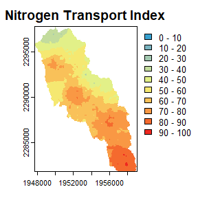
Convenience function: Build it all!
The workflow described above includes all the basic functionality.
Some users may wish to use nsink to calculate the base
layers for an N-Sink analysis and then build an application outside of
R. A convenience function that downloads all data, prepares, calculates
removal, and generates static maps has been included to facilitate this
type of analysis. The nsink_build() function requires a HUC
ID, coordinate reference system, and sampling density. An output folder
is also needed but has a default location. Optional arguments for
forcing a new download and playing a sound to signal when the build has
finished. Nothing returns to R, but all prepped data files and
.tif files are written into the output folder for use in
other applications.
niantic_huc_id <- nsink_get_huc_id("Niantic River")$huc_12
aea <- 5072
nsink_build(niantic_huc_id, aea, samp_dens = 900)