Fitting Spatial Stream Network Models to Large Data Sets and Making Predictions (i.e., Kriging)

Background

It can be challenging to fit SSN models to large data sets because the computation burden associated with estimating spatial covariance parameters increases exponentially with $n$, the sample size. Typically, it is only feasible to fit SSN2 models using the standard (i.e., traditional) approach for data sets having no more than a few thousand observations. Ver Hoef et al. (2023) proposed an approach called spatial indexing that can be used to fit SSN models having tens to hundreds of thousands of observations relatively quickly. Ver Hoef et al. (2023) and Dumelle et al. (2024) show that spatial indexing tends to approximate the standard solution very accurately at a fraction of the computational cost via several simulation studies and data analyses. Spatial indexing works by splitting the data up into smaller subsets ($n_{subset} << n$) and pooling spatial covariance parameters estimates across these subsets. This vignette aims to compare the standard approach and large data (i.e., spatial indexing) approach directly on a moderately sized data set, whereby the standard approach can be fit relatively quickly. In SSN2, spatial indexing is available via the local argument to ssn_lm() and ssn_glm().

Interestingly, the main computational burden associated with prediction at new locations is actually related to the size of the observed data ($n$), not the number of locations requiring prediction ($n_{pred})$. Ver Hoef et al. (2023) describe an approach to prediction at new locations using models fit to large (observed) data sets called local neighborhood prediction. Local neighborhood prediction subsets the observed data to include only the size observations most correlated with the location requiring prediction (where size is an integer). Typically, this subsetting is done separately for each prediction location. However, due to computational constraints associated with the hydrologic distance matrices required by SSN models, local neighborhood prediction in SSN2 subsets the observed data to the size observations most correlated (on average) with all locations requiring prediction. In SSN2, local neighborhood prediction is available via the local argument to predict() and augment().

Before proceeding, we load the SSN2 and ggplot2 R packages (which can all be installed directly from CRAN) by running:

library(SSN2)
library(ggplot2)

The `bugs` Data

The bugs data is an SSN object that contains macroinvertebrate data in the Lower Snake Basin. It can be downloaded via GitHub at this link. We read in bugs by running:

bugs <- ssn_import("bugs.ssn", predpts = "pred")

There are 549 observed sites ($n$) and 300 prediction sites ($n_{pred}$):

bugs
#> Object of class SSN
#> 
#> Object includes observations on 13 variables across 549 sites within the bounding box
#>     xmin     ymin     xmax     ymax 
#> -1765346  2459843 -1343175  2909567 
#> 
#> Object also includes 1 set of prediction points with 300 locations
#> 
#> Variable names are (found using ssn_names(object)):
#> $obs
#>  [1] "comid"     "ELEV_DEM"  "AREAWTMAP" "Rich"      "rid"       "ratio"    
#>  [7] "upDist"    "afvArea"   "locID"     "netID"     "pid"       "geometry" 
#> [13] "netgeom"  
#> 
#> $pred
#>  [1] "comid"     "ELEV_DEM"  "AREAWTMAP" "rid"       "ratio"     "upDist"   
#>  [7] "afvArea"   "locID"     "netID"     "pid"       "geom"      "netgeom"

We visualize the flowlines (edges), observed macroinvertebrate richness (obs), and prediction sites (preds) by running:

ggplot() +
  geom_sf(data = bugs$edges, linewidth = 0.1, alpha = 0.8, color = "darkgrey") +
  geom_sf(data = bugs$preds$pred, color = "black", size = 0.9) +
  geom_sf(data = bugs$obs, aes(color = Rich), size = 2) +
  scale_color_viridis_c(option = "H", limits = c(0, 59)) +
  theme_bw(base_size = 16)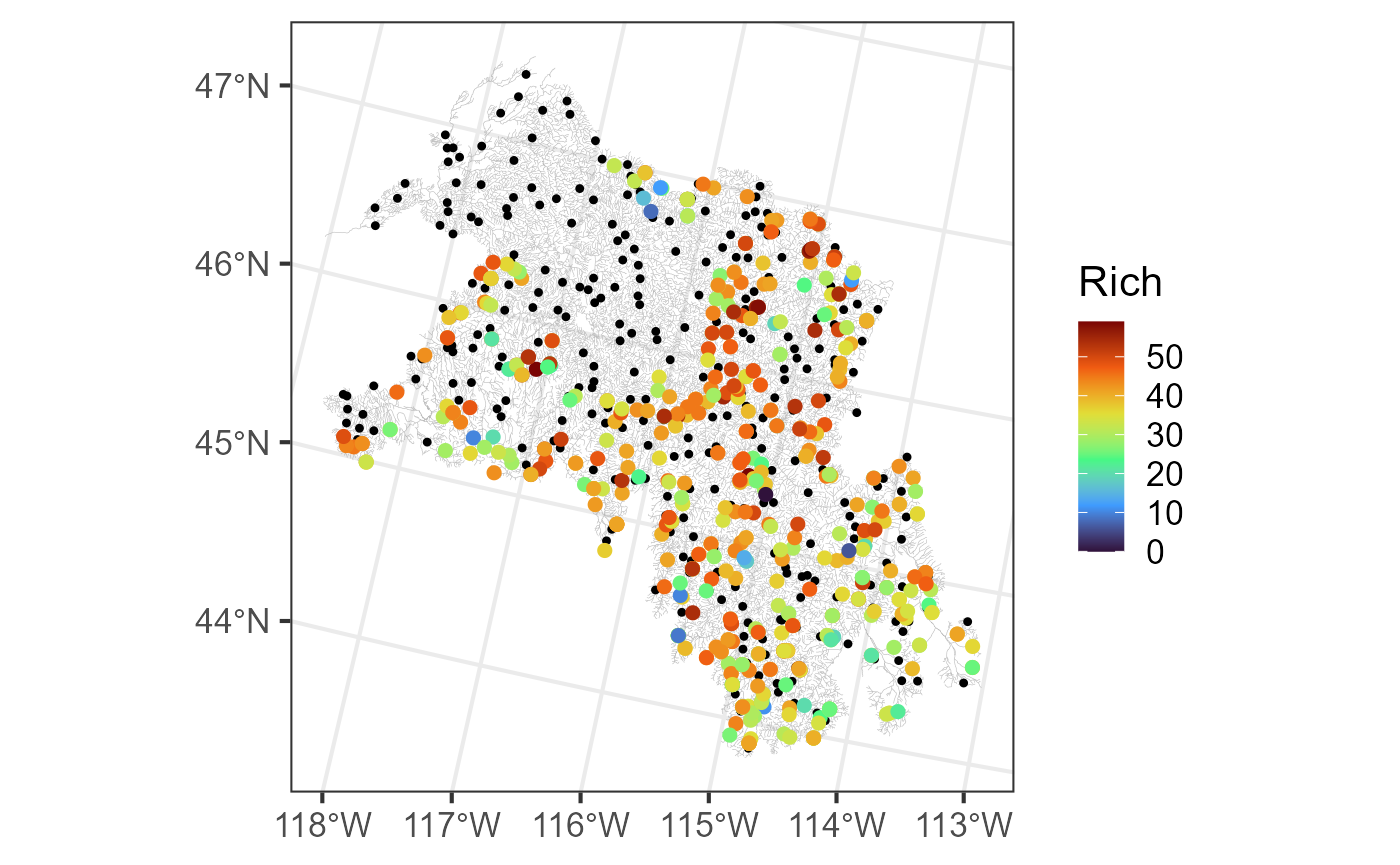

The Standard SSN Approach

Before fitting a standard SSN model to the bugs data, we create the hydrologic distance matrices required for model fitting by running:

ssn_create_distmat(bugs, predpts = "pred", among_predpts = TRUE)

Then we fit a standard SSN model by running:

standard_start <- Sys.time()
ssn_mod <- ssn_lm(
  formula = Rich ~ ELEV_DEM,
  ssn.object = bugs,
  tailup_type = "exponential",
  taildown_type = "exponential",
  additive = "afvArea"
)
standard_time <- Sys.time() - standard_start
standard_time
#> Time difference of 5.222182 secs

The model took 5.22 seconds to fit.

We augment the prediction data with predictions by running:

aug_ssn_mod <- augment(ssn_mod, newdata = "pred", interval = "prediction")

The Large Data SSN Approach (i.e., Spatial Indexing)

We create the hydrologic distance matrices required for fitting SSN models to large data sets via spatial indexing using ssn_create_bigdist():

ssn_create_bigdist(bugs, predpts = "pred", among_predpts = TRUE, no_cores = 2)

Like ssn_create_distmat(), ssn_create_bigdist() creates distance matrices in the distance folder of the .ssn. However, the distance matrices created by ssn_create_bigdist() have a special .bmat or .txt extension (instead of a .Rdata) extension. Distance matrices with .bmat and .txt extensions are accessed when we implement spatial indexing via the local argument:

set.seed(1)
bd_start <- Sys.time()
ssn_mod_bd <- ssn_lm(
  formula = Rich ~ ELEV_DEM,
  ssn.object = bugs,
  tailup_type = "exponential",
  taildown_type = "exponential",
  additive = "afvArea",
  local = TRUE
)
bd_time <- Sys.time() - bd_start
bd_time
#> Time difference of 2.370396 secs

The model took 2.37 seconds to fit.

The local argument set to TRUE implements default settings of a more complex local list that has several options controlling nuances of the spatial indexing. One of these options is the method used to assign observations to smaller subsets. The default approach is k-means clustering, chosen so that each smaller subset has a sample size of approximately 200. We can access the smaller subsets used by the model object and visualize them by running:

bugs$obs$index <- as.factor(ssn_mod_bd$local_index)
ggplot() +
  geom_sf(data = bugs$edges, linewidth = 0.1, alpha = 0.8, color = "darkgrey") +
  geom_sf(data = bugs$obs, aes(color = index), size = 2) +
  scale_color_viridis_d() +
  theme_bw(base_size = 16)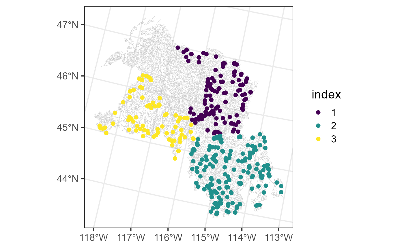

The kmeans() algorithm that determines subsets uses a random start, so setting a seed is required to reproduce results exactly. Model results should not change substantially between random starts, however. A fixed subset list can be provided to local so that subset assignment does not change across model fits. For more on the local argument, see the ssn_lm() documentation by running ?ssn_lm() or by visiting this link.

Now we use the model fit via spatial indexing to make local neighborhood predictions. In predict() (and augment()), the default value for the local neighborhood size is 4,000, which is larger than $n = 549$. However, if we set size to be 250 (instead of 4,000), we can illustrate some concepts behind local neighborhood prediction in SSN2 that will be useful when observed data sets are larger and size $<< n$.

When setting size to 250, the 250 observations sharing the highest average covariance with the prediction locations are used as the local neighborhood subset. We compute the covariance matrix between the prediction and observed locations by running:

cov_pred_by_obs <- covmatrix(ssn_mod_bd, newdata = "pred")
dim(cov_pred_by_obs)
#> [1] 300 549

We then find the average covariance between the prediction and observed locations by running:

avg_cov_with_obs <- colMeans(cov_pred_by_obs)

We then order these (largest covariance first), find indices corresponding to the 250 observations with the highest average covariance, and create a vector called Include, that has the value "Yes" if the observation is used in the local neighborhood subset and the value "No" if it is not:

cov_order <- order(avg_cov_with_obs, decreasing = TRUE)
largest_300 <- cov_order[1:250]
row_number <- seq(from = 1, to = NROW(bugs$obs))
bugs$obs$Include <- ifelse(row_number %in% largest_300, "Yes", "No")

We can visualize these designations by running:

ggplot() +
  geom_sf(data = bugs$edges, linewidth = 0.1, alpha = 0.8, color = "darkgrey") +
  geom_sf(data = bugs$preds$pred, color = "black", size = 0.9) +
  geom_sf(data = bugs$obs, aes(color = Include)) +
  theme_bw()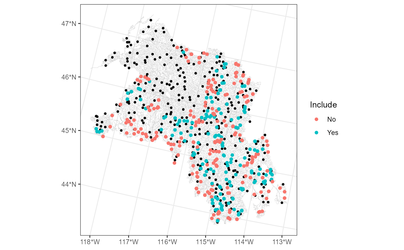

The 250 observations with the highest average covariance (Include = "Yes") tend to be nearby several prediction points, while the remaining observations (Include = "No") are often on the basin’s boundaries.

Using a local neighborhood size of 250, we then augment the prediction data with predictions by running:

aug_ssn_mod_bd <- augment(
  x = ssn_mod_bd,
  newdata = "pred",
  interval = "prediction",
  local = list(size = 250)
)

Unsurprisingly, the local neighborhood approach may not perform well when prediction locations are far away from any observed locations in the local neighborhood, which can happen when size $<< n$. In this case, one can separate prediction locations into smaller geographically based subsets and stored as separate prediction data sets in ssn.object$preds. The local neighborhood is recomputed for each subset separately based on the size observations most correlated (on average) with the prediction locations from that subset.

Comparing the Approaches

So far we fit the same model using the 1) standard and 2) large data set (i.e., spatial indexing) approaches and made predictions at new locations using the 1) standard and 2) large data set (i.e., local neighborhood prediction) approaches. How do the results from the distinct approaches compare?

Model Summaries

The two approaches have very similar summary output, particularly in the fixed effects coefficients table (which is often of primary ecological interest):

summary(ssn_mod)
#> 
#> Call:
#> ssn_lm(formula = Rich ~ ELEV_DEM, ssn.object = bugs, tailup_type = "exponential", 
#>     taildown_type = "exponential", additive = "afvArea")
#> 
#> Residuals:
#>     Min      1Q  Median      3Q     Max 
#> -36.387  -5.289   1.693   7.139  22.507 
#> 
#> Coefficients (fixed):
#>              Estimate Std. Error z value Pr(>|z|)    
#> (Intercept) 44.358544   2.216618  20.012  < 2e-16 ***
#> ELEV_DEM    -0.004651   0.001357  -3.428 0.000609 ***
#> ---
#> Signif. codes:  0 '***' 0.001 '**' 0.01 '*' 0.05 '.' 0.1 ' ' 1
#> 
#> Pseudo R-squared: 0.02134
#> 
#> Coefficients (covariance):
#>                 Effect     Parameter   Estimate
#>     tailup exponential  de (parsill)  5.281e+00
#>     tailup exponential         range  1.008e+06
#>   taildown exponential  de (parsill)  2.395e+01
#>   taildown exponential         range  4.582e+04
#>                 nugget        nugget  6.016e+01
summary(ssn_mod_bd)
#> 
#> Call:
#> ssn_lm(formula = Rich ~ ELEV_DEM, ssn.object = bugs, tailup_type = "exponential", 
#>     taildown_type = "exponential", additive = "afvArea", local = TRUE)
#> 
#> Residuals:
#>     Min      1Q  Median      3Q     Max 
#> -36.608  -5.439   1.572   6.845  22.290 
#> 
#> Coefficients (fixed):
#>              Estimate Std. Error z value Pr(>|z|)    
#> (Intercept) 44.198118   2.018556  21.896  < 2e-16 ***
#> ELEV_DEM    -0.004428   0.001255  -3.528 0.000418 ***
#> ---
#> Signif. codes:  0 '***' 0.001 '**' 0.01 '*' 0.05 '.' 0.1 ' ' 1
#> 
#> Pseudo R-squared: 0.02201
#> 
#> Coefficients (covariance):
#>                 Effect     Parameter   Estimate
#>     tailup exponential  de (parsill)  1.417e+00
#>     tailup exponential         range  9.174e+05
#>   taildown exponential  de (parsill)  2.496e+01
#>   taildown exponential         range  2.834e+04
#>                 nugget        nugget  5.888e+01

Leave-One-Out Cross Validation

The two approaches have very similar leave-one-out cross validation output:

loocv(ssn_mod)
#> # A tibble: 1 × 10
#>     bias std.bias  MSPE RMSPE std.MSPE   RAV  cor2 cover.80 cover.90 cover.95
#>    <dbl>    <dbl> <dbl> <dbl>    <dbl> <dbl> <dbl>    <dbl>    <dbl>    <dbl>
#> 1 0.0382  0.00959  75.3  8.68    0.984  8.74 0.157    0.825    0.903    0.953
loocv(ssn_mod_bd)
#> # A tibble: 1 × 10
#>     bias std.bias  MSPE RMSPE std.MSPE   RAV  cor2 cover.80 cover.90 cover.95
#>    <dbl>    <dbl> <dbl> <dbl>    <dbl> <dbl> <dbl>    <dbl>    <dbl>    <dbl>
#> 1 0.0340  0.00860  75.4  8.69     1.01  8.63 0.155    0.821    0.903    0.953

Prediction

The predictions from the two approaches are very similar. We see the first few rows of the augmented prediction data by running:

head(aug_ssn_mod[, c("ELEV_DEM", ".fitted", ".lower", ".upper", "pid")])
#> Simple feature collection with 6 features and 5 fields
#> Geometry type: POINT
#> Dimension:     XY
#> Bounding box:  xmin: -1752503 ymin: 2662140 xmax: -1682209 ymax: 2722702
#> Projected CRS: USA_Contiguous_Albers_Equal_Area_Conic_USGS_version
#> # A tibble: 6 × 6
#>   ELEV_DEM .fitted .lower .upper   pid           geometry
#>      <int>   <dbl>  <dbl>  <dbl> <int>        <POINT [m]>
#> 1      707    41.0   23.2   58.7   550 (-1682209 2720031)
#> 2     1266    38.4   19.9   56.9   709 (-1709066 2717244)
#> 3     1262    39.8   21.5   58.1   868 (-1752503 2692751)
#> 4      888    38.8   20.5   57.0  1141 (-1698700 2662140)
#> 5     1303    39.9   21.7   58.1  1365 (-1750463 2674396)
#> 6     1078    40.0   22.4   57.6  1613 (-1685728 2722702)
head(aug_ssn_mod_bd[, c("ELEV_DEM", ".fitted", ".lower", ".upper", "pid")])
#> Simple feature collection with 6 features and 5 fields
#> Geometry type: POINT
#> Dimension:     XY
#> Bounding box:  xmin: -1752503 ymin: 2662140 xmax: -1682209 ymax: 2722702
#> Projected CRS: USA_Contiguous_Albers_Equal_Area_Conic_USGS_version
#> # A tibble: 6 × 6
#>   ELEV_DEM .fitted .lower .upper   pid           geometry
#>      <int>   <dbl>  <dbl>  <dbl> <int>        <POINT [m]>
#> 1      707    41.4   23.5   59.2   550 (-1682209 2720031)
#> 2     1266    38.7   20.5   56.8   709 (-1709066 2717244)
#> 3     1262    39.6   21.6   57.7   868 (-1752503 2692751)
#> 4      888    40.4   22.2   58.6  1141 (-1698700 2662140)
#> 5     1303    39.8   21.8   57.8  1365 (-1750463 2674396)
#> 6     1078    40.7   23.2   58.1  1613 (-1685728 2722702)

We visualize the predictions from the standard approach and local neighborhood (LNBH) approach by running:

aug_ssn_mod$type <- "Standard"
aug_ssn_mod_bd$type <- "LNBH"
augs <- rbind(aug_ssn_mod, aug_ssn_mod_bd)
augs$type <- factor(augs$type, levels = c("Standard", "LNBH"))
ggplot(augs) +
  geom_sf(data = bugs$edges, linewidth = 0.1, alpha = 0.8, color = "darkgrey") +
  geom_sf(data = augs, aes(color = .fitted), size = 2) +
  facet_wrap(~ type) +
  scale_color_viridis_c(option = "H", limits = c(0, 59)) +
  scale_x_continuous(breaks = -c(117, 114)) +
  theme_bw(base_size = 16)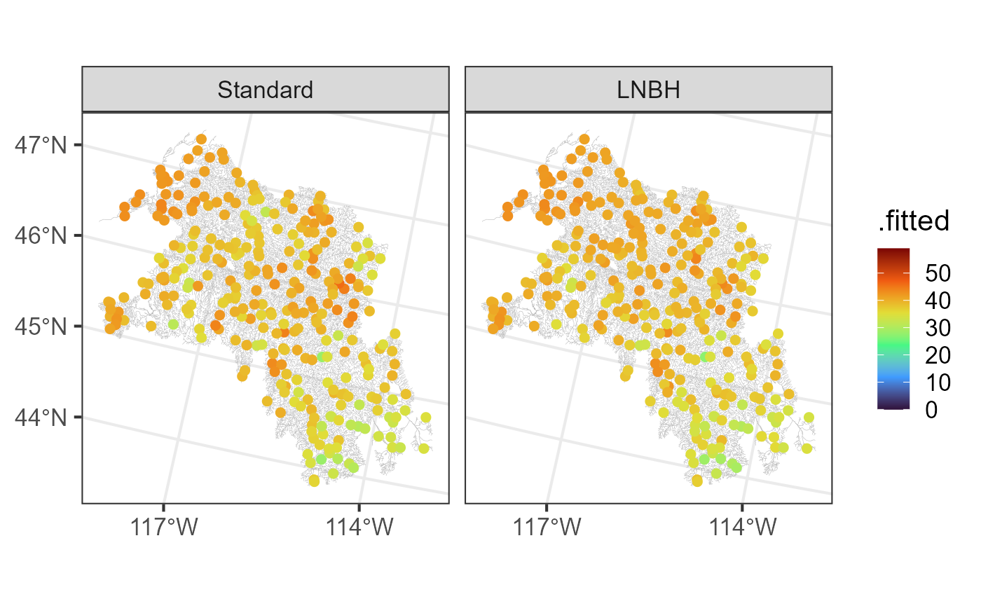

We predict the average in the entire domain (i.e., block prediction) by running:

predict(
  object = ssn_mod,
  newdata = "pred",
  block = TRUE,
  interval = "prediction"
)
#>        fit      lwr      upr
#> 1 38.44282 36.94272 39.94292
predict(
  object = ssn_mod_bd,
  newdata = "pred",
  block = TRUE,
  interval = "prediction",
  local = list(size = 250)
)
#>        fit      lwr      upr
#> 1 38.63474 37.08141 40.18807

Closing Thoughts

The standard and large data set (i.e., spatial indexing; local neighborhood prediction) approaches used here yielded very similar results. For data with larger observed sample sizes ($n > \approx 5,000$), the spatial indexing and local neighborhood prediction approaches are significantly more computationally efficient than their standard approach counterparts (in fact, the standard approaches won’t be feasible for very large data sets). See Ver Hoef et al. (2023) and Dumelle et al. (2024) for a more thorough look at spatial indexing and local neighborhood prediction.

Why the Computational Burden?

The main computational burden associated with estimation and prediction is computing products that involve the inverse covariance matrix. Inversion scales cubically with the sample size. This means that if the sample size doubles, the inversion computational cost increases eight-fold! For estimating parameters, this inversion is required during each step of the optimization algorithm (generally, dozens of steps are required for convergence of the optimization algorithm). For prediction, this inversion is only required once. So, for data sets having a few thousand observations, one can use spatial indexing to fit the model but then use standard prediction instead of local neighborhood prediction (as the inverse covariance matrix products are only required once).

R Code Appendix

knitr::opts_chunk$set(
  collapse = TRUE,
  comment = "#>",
  message = FALSE,
  warning = FALSE
)
library(SSN2)
library(ggplot2)
bugs <- ssn_import("bugs.ssn", predpts = "pred")
bugs
ggplot() +
  geom_sf(data = bugs$edges, linewidth = 0.1, alpha = 0.8, color = "darkgrey") +
  geom_sf(data = bugs$preds$pred, color = "black", size = 0.9) +
  geom_sf(data = bugs$obs, aes(color = Rich), size = 2) +
  scale_color_viridis_c(option = "H", limits = c(0, 59)) +
  theme_bw(base_size = 16)
ssn_create_distmat(bugs, predpts = "pred", among_predpts = TRUE)
standard_start <- Sys.time()
ssn_mod <- ssn_lm(
  formula = Rich ~ ELEV_DEM,
  ssn.object = bugs,
  tailup_type = "exponential",
  taildown_type = "exponential",
  additive = "afvArea"
)
standard_time <- Sys.time() - standard_start
standard_time
aug_ssn_mod <- augment(ssn_mod, newdata = "pred", interval = "prediction")
ssn_create_bigdist(bugs, predpts = "pred", among_predpts = TRUE, no_cores = 2)
set.seed(1)
bd_start <- Sys.time()
ssn_mod_bd <- ssn_lm(
  formula = Rich ~ ELEV_DEM,
  ssn.object = bugs,
  tailup_type = "exponential",
  taildown_type = "exponential",
  additive = "afvArea",
  local = TRUE
)
bd_time <- Sys.time() - bd_start
bd_time
bugs$obs$index <- as.factor(ssn_mod_bd$local_index)
ggplot() +
  geom_sf(data = bugs$edges, linewidth = 0.1, alpha = 0.8, color = "darkgrey") +
  geom_sf(data = bugs$obs, aes(color = index), size = 2) +
  scale_color_viridis_d() +
  theme_bw(base_size = 16)
cov_pred_by_obs <- covmatrix(ssn_mod_bd, newdata = "pred")
dim(cov_pred_by_obs)
avg_cov_with_obs <- colMeans(cov_pred_by_obs)
cov_order <- order(avg_cov_with_obs, decreasing = TRUE)
largest_300 <- cov_order[1:250]
row_number <- seq(from = 1, to = NROW(bugs$obs))
bugs$obs$Include <- ifelse(row_number %in% largest_300, "Yes", "No")
ggplot() +
  geom_sf(data = bugs$edges, linewidth = 0.1, alpha = 0.8, color = "darkgrey") +
  geom_sf(data = bugs$preds$pred, color = "black", size = 0.9) +
  geom_sf(data = bugs$obs, aes(color = Include)) +
  theme_bw()
aug_ssn_mod_bd <- augment(
  x = ssn_mod_bd,
  newdata = "pred",
  interval = "prediction",
  local = list(size = 250)
)
summary(ssn_mod)
summary(ssn_mod_bd)
loocv(ssn_mod)
loocv(ssn_mod_bd)
head(aug_ssn_mod[, c("ELEV_DEM", ".fitted", ".lower", ".upper", "pid")])
head(aug_ssn_mod_bd[, c("ELEV_DEM", ".fitted", ".lower", ".upper", "pid")])
aug_ssn_mod$type <- "Standard"
aug_ssn_mod_bd$type <- "LNBH"
augs <- rbind(aug_ssn_mod, aug_ssn_mod_bd)
augs$type <- factor(augs$type, levels = c("Standard", "LNBH"))
ggplot(augs) +
  geom_sf(data = bugs$edges, linewidth = 0.1, alpha = 0.8, color = "darkgrey") +
  geom_sf(data = augs, aes(color = .fitted), size = 2) +
  facet_wrap(~ type) +
  scale_color_viridis_c(option = "H", limits = c(0, 59)) +
  scale_x_continuous(breaks = -c(117, 114)) +
  theme_bw(base_size = 16)
predict(
  object = ssn_mod,
  newdata = "pred",
  block = TRUE,
  interval = "prediction"
)
predict(
  object = ssn_mod_bd,
  newdata = "pred",
  block = TRUE,
  interval = "prediction",
  local = list(size = 250)
)

References

Dumelle, Michael, Jay M Ver Hoef, Amalia Handler, Ryan A Hill, Matt Higham, and Anthony R Olsen. 2024. “Modeling Lake Conductivity in the Contiguous United States Using Spatial Indexing for Big Spatial Data.” Spatial Statistics 59: 100808.

Ver Hoef, Jay M, Michael Dumelle, Matt Higham, Erin E Peterson, and Daniel J Isaak. 2023. “Indexing and Partitioning the Spatial Linear Model for Large Data Sets.” Plos One 18 (11): e0291906.

Michael Dumelle