4  Advanced Applications

We’ll explore a few ‘advanced’ applications in this section, exploring the use of web services, exploring some means of using STAC resources in R, using R extensions, and some spatial modeling libraries

4.1 Goals and Outcomes

• Gain familiarity with using web services for several applications in R
• Learn about using STAC resources in R
• Know about several extensions for integrating with other GIS software and tools in R
• Gain some familiarity with spatial sampling and modeling libraries

Throughout this section we’ll use the following packages:

library(AOI)
library(nhdplusTools)
library(dataRetrieval)
library(mapview)
mapviewOptions(fgb=FALSE)
library(ggplot2)
library(StreamCatTools)
library(tmap)
library(opendap.catalog)
library(climateR)
library(terra)
library(zonal)
library(cowplot)
library(spsurvey)
library(spmodel)

4.2 Using Web Services

4.2.1 Hydrology data with nhdplusTools and dataRetrieval

Working with spatial data in R has been enhanced recently with packages that provide web-based subsetting services. We’ll walk through examples of several with a hydrological focus.

We previously saw an example of getting an area of interest using Mike Johnson’s handy AOI package, and we saw an example of getting hydrology data using the dataRetrieval package which leverages the underlying Network-Linked Data Index (NLDI) service.

Here we’ll demonstrate leveraging the same service through the nhdplusTools package in combination with the AOI package to quickly pull in spatial data for analysis via web services and combine with gage data from the dataRetrieval package.

You can read a concise background on using web services in R here

corvallis <- get_nhdplus(aoi_get("Corvallis, OR"), realization = "all")
# get stream gages too
corvallis$gages <- nhdplusTools::get_nwis(aoi_get("Corvallis, OR"))
mapview(corvallis)

Pretty cool. All that data in a one-liner!

Next we’ll go back to the South Santiam basin we derived in the geoprocessing section and we’ll grab all the gage data in the basin. We’ll get stream flow data for the gages using dataRetrieval flow data in dataRetrieval is accessed with code ‘00060’ which can be found with dataRetrieval::parameterCdFile. See the dataRetrieval package website for documentation and tutorials.

nldi_feature <- list(featureSource = "nwissite", 
                     featureID = "USGS-14187200")
SouthSantiam <- navigate_nldi(nldi_feature,  mode = "upstreamTributaries", distance_km=100)
basin <- nhdplusTools::get_nldi_basin(nldi_feature = nldi_feature)

gages <- nhdplusTools::get_nwis(basin)
mapview(SouthSantiam) + mapview(basin) + mapview(gages)

Notice we pulled in some stream gages within the bounding box of our basin but not within the watershed - let’s fix that with st_intersection:

gages <- sf::st_intersection(gages, basin)
mapview(SouthSantiam) + mapview(basin) + mapview(gages)

Now we’ll grab stream flow data for our watershed with dataRetrieval:

flows = dataRetrieval::readNWISdv(site = gages$site_no, parameterCd = "00060") |> 
  renameNWISColumns()

ggplot(data = flows) + 
  geom_line(aes(x = Date, y = Flow)) + 
  facet_wrap('site_no')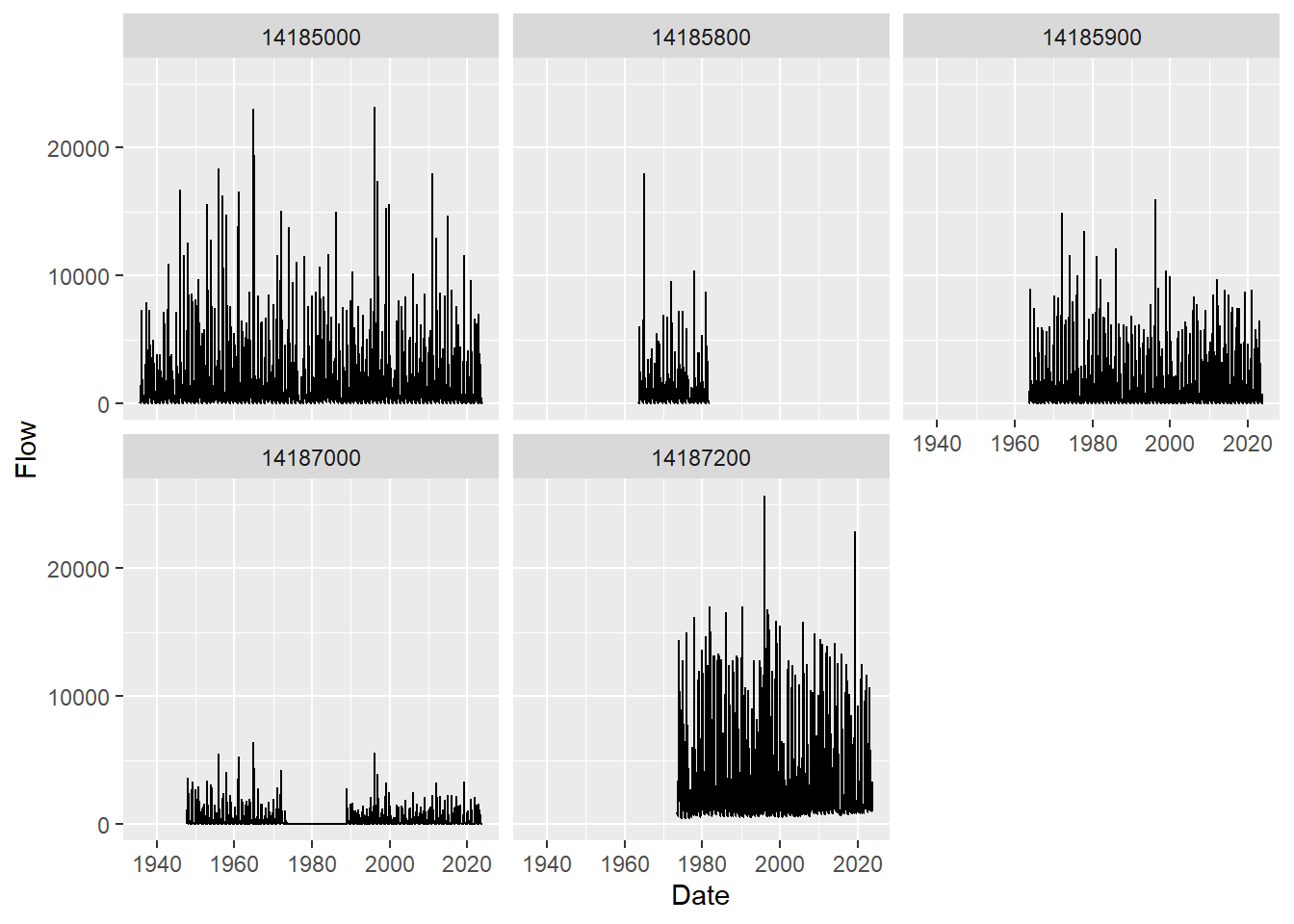

It looks like only 5 of our nwis sites had flow data for which we’ve plotted streamflow information for all the years available.

We’ve shown the client functionality for The Network-Linked Data Index (NLDI) using both nhdplusTools and dataRetrieval; either works similarly. The NLDI can index spatial and river network-linked data and navigate the river network to allow discovery of indexed information.

To use the NLDI you supply a starting feature which can be an:

• NHDPlus COMID
• NWIS ID
• WQP ID
• several other feature identifiers

You can see what is available with:

knitr::kable(dataRetrieval::get_nldi_sources())

source	sourceName	features
ca_gages	Streamgage catalog for CA SB19	https://labs.waterdata.usgs.gov/api/nldi/linked-data/ca_gages
census2020-nhdpv2	2020 Census Block - NHDPlusV2 Catchment Intersections	https://labs.waterdata.usgs.gov/api/nldi/linked-data/census2020-nhdpv2
epa_nrsa	EPA National Rivers and Streams Assessment	https://labs.waterdata.usgs.gov/api/nldi/linked-data/epa_nrsa
geoconnex-demo	geoconnex contribution demo sites	https://labs.waterdata.usgs.gov/api/nldi/linked-data/geoconnex-demo
gfv11_pois	USGS Geospatial Fabric V1.1 Points of Interest	https://labs.waterdata.usgs.gov/api/nldi/linked-data/gfv11_pois
huc12pp	HUC12 Pour Points	https://labs.waterdata.usgs.gov/api/nldi/linked-data/huc12pp
nmwdi-st	New Mexico Water Data Initative Sites	https://labs.waterdata.usgs.gov/api/nldi/linked-data/nmwdi-st
npdes	NPDES Facilities that Discharge to Water	https://labs.waterdata.usgs.gov/api/nldi/linked-data/npdes
nwisgw	NWIS Groundwater Sites	https://labs.waterdata.usgs.gov/api/nldi/linked-data/nwisgw
nwissite	NWIS Surface Water Sites	https://labs.waterdata.usgs.gov/api/nldi/linked-data/nwissite
ref_gage	geoconnex.us reference gages	https://labs.waterdata.usgs.gov/api/nldi/linked-data/ref_gage
vigil	Vigil Network Data	https://labs.waterdata.usgs.gov/api/nldi/linked-data/vigil
wade	Water Data Exchange 2.0 Sites	https://labs.waterdata.usgs.gov/api/nldi/linked-data/wade
WQP	Water Quality Portal	https://labs.waterdata.usgs.gov/api/nldi/linked-data/wqp
comid	NHDPlus comid	https://labs.waterdata.usgs.gov/api/nldi/linked-data/comid

4.2.2 Watershed data with StreamCatTools

StreamCatTools is an R package I’ve written that provides a client for the API for the StreamCat dataset, a comprehensive set of watershed data for the NHDPlus.

We can easily pull in watershed data from StreamCat for our basin with StreamCatTools:

comids <- SouthSantiam$UT_flowlines$nhdplus_comid
# we need a simple comma separated list for StreamCat
comids <- paste(comids,collapse=",",sep="")

df <- StreamCatTools::sc_get_data(metric='MSST_2014', aoi='other', comid=comids)

flowlines <- SouthSantiam$UT_flowlines
flowlines$MSST_2014 <- df$MSST_2014[match(flowlines$nhdplus_comid, df$COMID)]
# drop any NAs
flowlines <- flowlines |> dplyr::filter(!is.na(flowlines$MSST_2014))

tm_shape(flowlines) + tm_lines("MSST_2014", title.col ="Mean Summer Stream\nTemperature (deg C) 2014")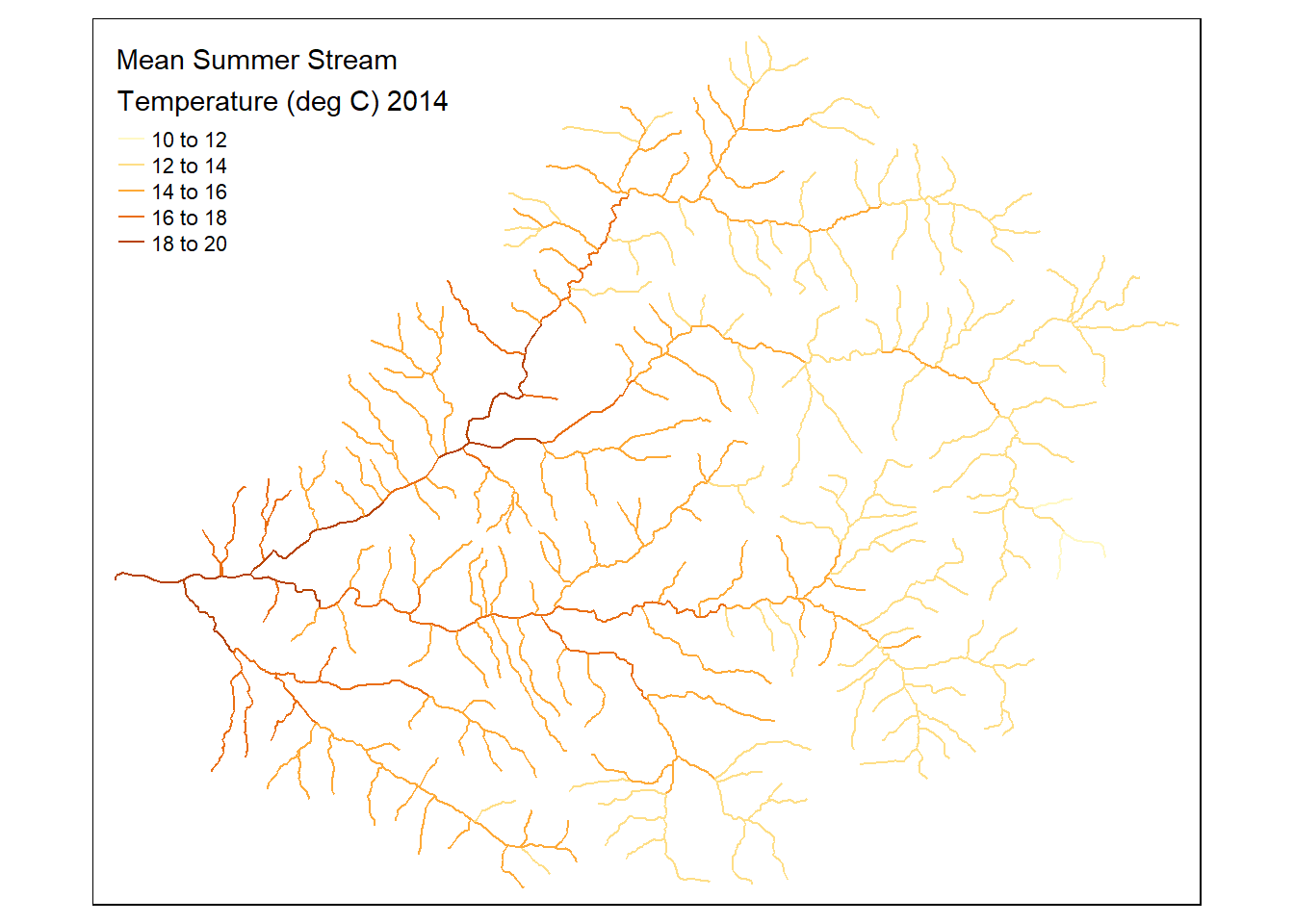 

4.2.3 Elevation as a service

Thanks to our own Jeff Hollister we have the handy elevatr package for retrieving elevation data as a service for user provided points or areas - we can easily return elevation for our South Santiam basin we’ve created using elevation web services with elevatr:

elev <- elevatr::get_elev_raster(basin, z = 9)

Mosaicing & Projecting

Note: Elevation units are in meters.

mapview(elev)

Warning in rasterCheckSize(x, maxpixels = maxpixels): maximum number of pixels for Raster* viewing is 5e+05 ; 
the supplied Raster* has 991200 
 ... decreasing Raster* resolution to 5e+05 pixels
 to view full resolution set 'maxpixels =  991200 '

4.2.4 OpenDAP and STAC

OPeNDAP allows us to access geographic or temporal slices of massive datasets over HTTP via web services. STAC similarly is a specification that allows us to access geospatial assets via web services. Using STAC you can access a massive trove of resources on Microsoft Planetary Computer via the rstac package as in examples here.

Here we’ll just show an example of using OpenDAP via Mike Johnson’s OpenDAP Catalog and ClimateR packages.

# See what is available - a LOT! As in 14,691 resources available via web services!!
dplyr::glimpse(opendap.catalog::params)

Rows: 14,691
Columns: 15
$ id        <chr> "hawaii_soest_1727_02e2_b48c", "hawaii_soest_1727_02e2_b48c"…
$ grid_id   <chr> "73", "73", "73", "73", "73", "73", "73", "73", "73", "73", …
$ URL       <chr> "https://apdrc.soest.hawaii.edu/erddap/griddap/hawaii_soest_…
$ tiled     <chr> "", "", "", "", "", "", "", "", "", "", "", "", "", "", "", …
$ variable  <chr> "nudp", "nusf", "nuvdp", "nuvsf", "nvdp", "nvsf", "sudp", "s…
$ varname   <chr> "nudp", "nusf", "nuvdp", "nuvsf", "nvdp", "nvsf", "sudp", "s…
$ long_name <chr> "number of deep zonal velocity profiles", "number of surface…
$ units     <chr> NA, NA, NA, NA, NA, NA, NA, NA, NA, NA, NA, NA, NA, NA, NA, …
$ model     <chr> NA, NA, NA, NA, NA, NA, NA, NA, NA, NA, NA, NA, NA, NA, NA, …
$ ensemble  <chr> NA, NA, NA, NA, NA, NA, NA, NA, NA, NA, NA, NA, NA, NA, NA, …
$ scenario  <chr> NA, NA, NA, NA, NA, NA, NA, NA, NA, NA, NA, NA, NA, NA, NA, …
$ T_name    <chr> "time", "time", "time", "time", "time", "time", "time", "tim…
$ duration  <chr> "2001-01-01/2022-01-01", "2001-01-01/2022-01-01", "2001-01-0…
$ interval  <chr> "365 days", "365 days", "365 days", "365 days", "365 days", …
$ nT        <dbl> 22, 22, 22, 22, 22, 22, 22, 22, 22, 22, 22, 22, 22, 22, 22, …

We can search for resources of interest:

opendap.catalog::search("monthly swe")

# A tibble: 15 × 16
   id        grid_id URL   tiled variable varname long_name units model ensemble
   <chr>     <chr>   <chr> <chr> <chr>    <chr>   <chr>     <chr> <chr> <chr>   
 1 GLDAS     139     http… ""    swe_inst swe_in… "** snow… <NA>  CLSM… <NA>    
 2 GLDAS     139     http… ""    swe_inst swe_in… "** snow… <NA>  CLSM… <NA>    
 3 GLDAS     135     http… ""    swe_inst swe_in… "** snow… <NA>  NOAH… <NA>    
 4 GLDAS     135     http… ""    swe_inst swe_in… "** snow… <NA>  NOAH… <NA>    
 5 GLDAS     139     http… ""    swe_inst swe_in… "** snow… <NA>  NOAH… <NA>    
 6 GLDAS     139     http… ""    swe_inst swe_in… "** snow… <NA>  NOAH… <NA>    
 7 GLDAS     139     http… ""    swe_inst swe_in… "** snow… <NA>  VIC10 <NA>    
 8 GLDAS     139     http… ""    swe_inst swe_in… "** snow… <NA>  VIC10 <NA>    
 9 NLDAS     174     http… ""    swe      swe     "snow wa… kg m… MOS0… <NA>    
10 NLDAS     174     http… ""    swe      swe     "snow wa… kg m… NOAH… <NA>    
11 NLDAS     174     http… ""    swe      swe     "snow wa… kg m… VIC0… <NA>    
12 terracli… 116     http… ""    swe      swe     "snow_wa… mm    <NA>  <NA>    
13 terracli… 116     http… ""    swe      swe     "snow_wa… mm    <NA>  <NA>    
14 terracli… 116     http… ""    swe      swe     "snow_wa… mm    <NA>  <NA>    
15 terracli… 116     http… ""    swe      swe     "snow_wa… mm    <NA>  <NA>    
# ℹ 6 more variables: scenario <chr>, T_name <chr>, duration <chr>,
#   interval <chr>, nT <dbl>, rank <dbl>

And we can extract a particular resource (in this case PRISM climate data) using climateR - we’ll go back to using our counties in Oregon data from earlier.

counties <- aoi_get(state='Oregon', county='all')
precip <- getPRISM(counties,
               varname = "ppt",
               startDate = "2020-01-01",
               endDate  = "2020-03-30",
               timeRes="monthly")
precip <- terra::rast(precip)

names(precip)

[1] "ppt_2020-01-01"          "ppt_2020-01-31 08:00:00"
[3] "ppt_2020-03-01 16:00:00" "ppt_2020-04-01"         

plot(precip)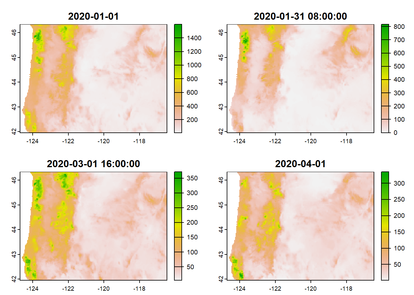

4.3 Zonal Statistics

We can easily run zonal statistics for counties of Oregon using the zonal package with our precipitation data we extracted for Oregon from PRISM:

counties <- sf::st_transform(counties, crs(precip))
county_precip <- zonal::execute_zonal(precip, counties, ID='name',fun='mean')

# Rename monthly precip
names(county_precip)[16:17] <- c('ppt_2020-01-31','ppt_2020-03-01')
a <- ggplot() + 
  geom_sf(data=county_precip, aes(fill=`ppt_2020-01-01`))
b <- ggplot() + 
  geom_sf(data=county_precip, aes(fill=`ppt_2020-01-31`))
c <- ggplot() + 
  geom_sf(data=county_precip, aes(fill=`ppt_2020-03-01`))
d <- ggplot() + 
  geom_sf(data=county_precip, aes(fill=`ppt_2020-04-01`))
plot_grid(a,b,c,d)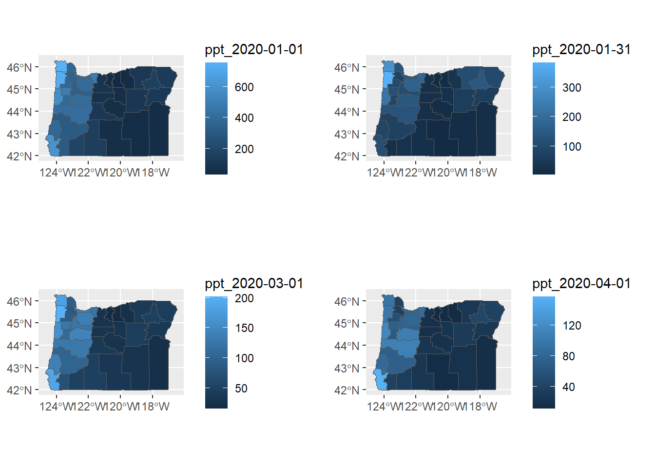

4.4 Extensions

4.4.1 RQGIS

There’s a bit of overhead to install QGIS and configure RQGIS - I use QGIS but have not set up RQGIS myself, I recommend reading the description in Geocomputation with R

4.4.2 R-ArcGIS bridge

See this description describing how to link your R install to the R-ArcGIS bridge

4.4.3 Accessing Python toolbox using reticulate

I highly recommend this approach if you want to integrate python workflows and libraries (including arcpy) with R workflows within reproducible R quarto or markdown files.

library(reticulate)

We can immediately start playing with python within a code block designated as python

import pandas as pd

print('hello python')

some_dict = {'a':1, 'b':2, 'c':3}

print(some_dict.keys())

Load our gage data in Python…

import pandas as pd
gages = pd.read_csv('C:/Users/mweber/GitProjects/Rspatialworkshop/inst/extdata/Gages_flowdata.csv')
gages.head()
gages['STATE'].unique()
PNW_gages = gages[gages['STATE'].isin(['OR','WA','ID'])]

4.4.3.1 Access Python objects directly from R

Now work with the pandas data directly within R

gages <- st_as_sf(py$PNW_gages,coords = c('LON_SITE','LAT_SITE'),crs = 4269) 
gages <- st_transform(gages, crs=5070) #5070 is Albers system in metres
ggplot(gages) + geom_sf()

And share spatial results from Python You can work with spatial tools in Python and share results with R!

from rasterstats import zonal_stats
clnp = 'C:/Users/mweber/Temp/CraterLake_tm.shp'
elev = 'C:/Users/mweber/Temp/elevation_tm.tif'

park_elev = zonal_stats(clnp, elev, all_touched=True,geojson_out=True, stats="count mean sum nodata")
geostats = gp.GeoDataFrame.from_features(park_elev)

zonal <- py$geostats

4.4.4 R Whitebox Tools

We won’t go into here but worth mentioning as a rich set of tools you can access in R - whiteboxR

4.4.5 rgee

Here I’m just running the demo code in the ReadMe for the rgee package as a proof of concept of cool things you can do being able to leverage Earth Engine directly in R. Note that there is overhead in getting this all set up.

library(reticulate)
library(rgee)
ee_Initialize()
# gm <- import("geemap")

Function to create a time band containing image date as years since 1991.

createTimeBand <-function(img) {
  year <- ee$Date(img$get('system:time_start'))$get('year')$subtract(1991L)
  ee$Image(year)$byte()$addBands(img)
}

Using Earth Engine syntax, we ‘Map’ the time band creation helper over the night-time lights collection.

collection <- ee$
  ImageCollection('NOAA/DMSP-OLS/NIGHTTIME_LIGHTS')$
  select('stable_lights')$
  map(createTimeBand)

We compute a linear fit over the series of values at each pixel, visualizing the y-intercept in green, and positive/negative slopes as red/blue.

col_reduce <- collection$reduce(ee$Reducer$linearFit())
col_reduce <- col_reduce$addBands(
  col_reduce$select('scale'))
ee_print(col_reduce)

We make an interactive visualization - pretty cool!

Map$setCenter(9.08203, 47.39835, 3)
Map$addLayer(
  eeObject = col_reduce,
  visParams = list(
    bands = c("scale", "offset", "scale"),
    min = 0,
    max = c(0.18, 20, -0.18)
  ),
  name = "stable lights trend"
)

4.5 Spatial Sampling and Modeling

4.5.1 Spatial Sampling

Often we take a sample from a population and use the sample to make inferences regarding the population. For spatial resources, spatially balanced sampling generally yields samples that a more well-spread in space and representative of the true population compared to a sample that ignores spatial information. The spsurvey R package is used to select spatially balanced samples of sf objects using the Generalized Random Tessellation Stratified (GRTS) algorithm, which can be applied to POINT, LINESTRING, and POLYGON geometries.

The NE_Lakes data in spsurvey is an sf object with data on 195 lakes in the Northeastern United States. TO select a spatially balanced sample of size 50 from these 195 lakes, run

samp <- grts(NE_Lakes, 50)

The sample locations can be visualized alongside NE_Lakes by running

plot(samp, NE_Lakes, pch = 19, key.pos = 1)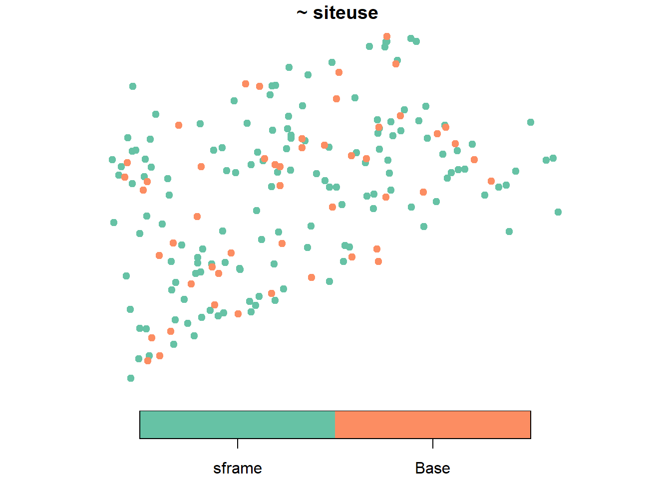

There are many additional options for sampling, such as stratification, unequal probability sampling, over/replacement sampling, and much more. spsurvey also has much more functionality, including tools for calculating the spatial balance of a sample and summarizing, visualizing, and analyzing data. To learn more about spsurvey, visit its website here.

4.5.2 Spatial Modeling

Linear models are used to describe the relationship between a response variable and explanatory variables. Linear models are typically fit in R using lm(). These models, however, ignore the fact that observations may be correlated in space. The spmodel R package provides support for fitting spatial linear models, which do explicitly incorporate spatial covariance/correlation. Spatial linear models are fit using the splm() function and share similar structure as lm().

The moss data in spmodel contains data on Zinc concentrations in Alaska, USA. The log Zinc concentration is visualized by running

ggplot(moss, aes(color = log_Zn)) +
  geom_sf() +
  scale_color_viridis_c()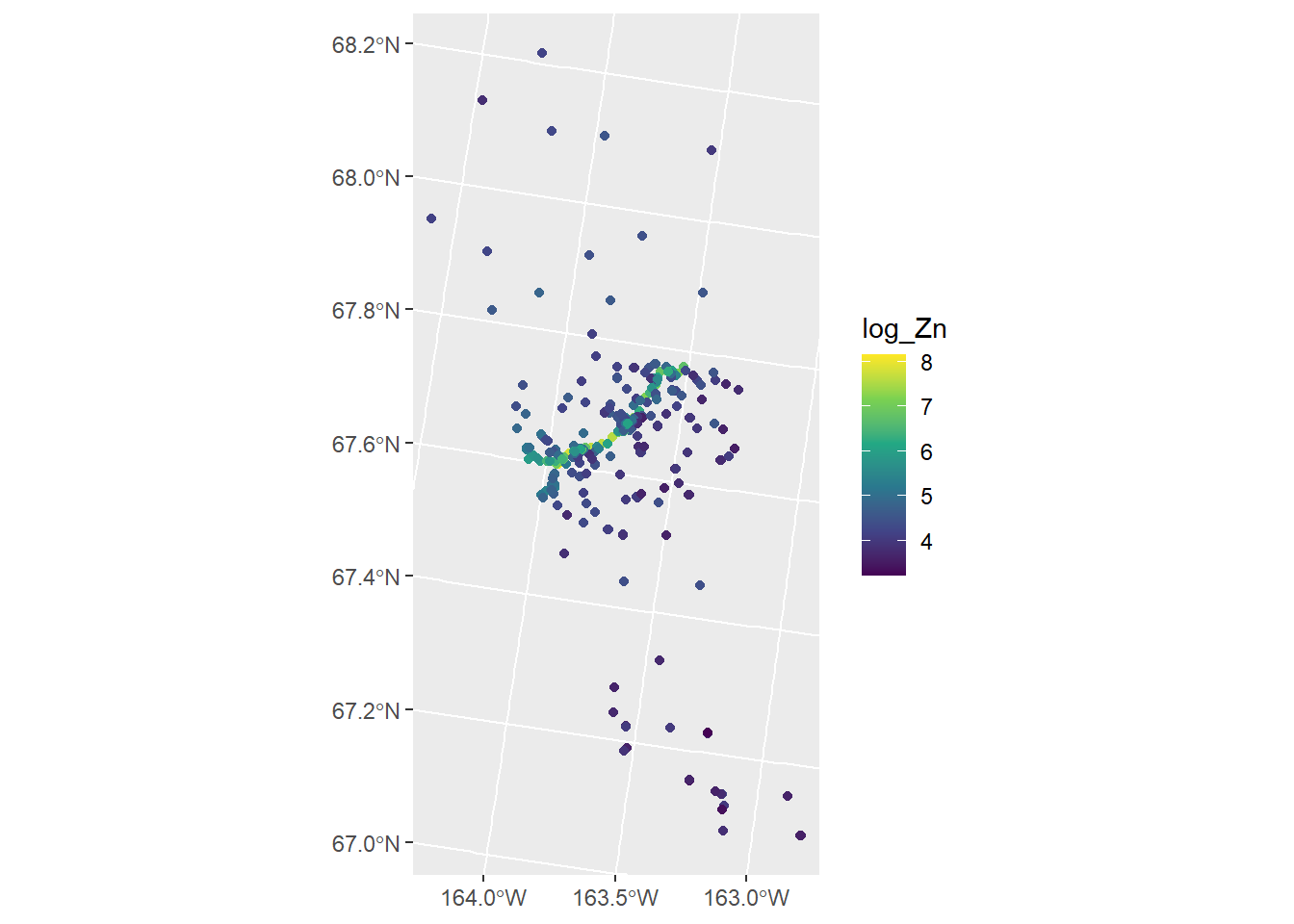

There is a road running through the middle of the domain where log Zinc concentrations are highest. We model log zinc concentration as a function of the log distance to the road with an exponential spatial covariance function by running

spmod <- splm(log_Zn ~ log_dist2road, moss, spcov_type = "exponential")
summary(spmod)

Call:
splm(formula = log_Zn ~ log_dist2road, data = moss, spcov_type = "exponential")

Residuals:
    Min      1Q  Median      3Q     Max 
-2.6801 -1.3606 -0.8103 -0.2485  1.1298 

Coefficients (fixed):
              Estimate Std. Error z value Pr(>|z|)    
(Intercept)    9.76825    0.25216   38.74   <2e-16 ***
log_dist2road -0.56287    0.02013  -27.96   <2e-16 ***
---
Signif. codes:  0 '***' 0.001 '**' 0.01 '*' 0.05 '.' 0.1 ' ' 1

Pseudo R-squared: 0.683

Coefficients (exponential spatial covariance):
       de        ie     range 
3.595e-01 7.897e-02 8.237e+03 

There appears to be a significant decrease in log zinc concentration as the log distance to the road increases. We can fit a non-spatial model and comapre both models using glances():

lmod <- splm(log_Zn ~ log_dist2road, moss, spcov_type = "none")
glances(spmod, lmod)

# A tibble: 2 × 10
  model     n     p  npar value   AIC  AICc logLik deviance pseudo.r.squared
  <chr> <int> <dbl> <int> <dbl> <dbl> <dbl>  <dbl>    <dbl>            <dbl>
1 spmod   365     2     3  367.  373.  373.  -184.     363.            0.683
2 lmod    365     2     1  634.  636.  636.  -317.     363.            0.671

The spatial model (spmod) has a much lower AIC and AICc than the non-spatial model (lmod), which indicates that incorporating spatial covariance/correlation into the model is quite helpful. To learn more about spmodel, visit its website here.

4.5.3 Spatial Stream Networks

The statistical modeling in spmodel uses Euclidean distances to measure spatial correlation. On a stream network, Euclidean distance (on its own) does not sufficiently describe proximity relationships. Spatial stream network models incorporate in-stream distance and Euclidean distance to improve model fit. The SSN R package has been available on CRAN for the last decade or so, but it was recently removed alongside the archiving of rgdal, rgeos, and maptools (see Resources) . SSN2 will be released on CRAN, very likely by the end of 2023, so keep an eye out for it!