3 Geoprocessing
We’ll explore a number operations in this section that make up what most of us probably think of as typical GIS operations and how to perform them in R - operations such as clipping, subsetting, joining, dissolving, performing map algebra.
Keep in mind as we mentioned earlier that sf contains functions that bind to these three primary underlying libraries:
- GDAL for reading and writing data
- GEOS for geometrical operations
- PRØJ for projection conversions and datum transformations
3.1 Goals and Outcomes
- Learn about fundamental spatial operations in R using spatial predicates in
sffor:- subsetting
- spatial join
- buffer
- logical set operations - union / intersection
- clipping
- generating centroids and ‘casting’ to other geometry types
- raster operations
- map algebra
- cropping and masking
- zonal operations
- Explore performing ‘map algebra’ type operations with raster data in R
- Learn how to do extract and zonal operations in R
Throughout this section we’ll use the following packages:
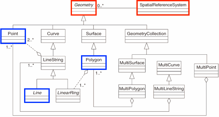
3.2 Operations on Geometries
This breakdown of simple features follows for the most part this section in Spatial Data Science
Simple and valid geometries
- Certain conditions have to be met with simple features:
- For linestrings to be considered simple they must not self-intersect:
LINESTRING (0 0, 1 1, 2 2, 0 2, 1 1, 2 0)
is_simple
FALSE -
For polygons several other conditions have to be met to be simple:
- polygon rings are closed (the lastpoint equals the first)
- polygon holes (inner rings) are inside their exterior ring
- polygon inner rings maximally touch the exterior ring in single points, not over a line
- a polygon ring does not repeat its own path
- in a multi-polygon, an external ring maximally touches another exterior ring in single points, not over a line
We can break down operations on geometries for vector features in the following way:
-
predicates: a logical asserting a certain property is
TRUE - measures: a quantity (a numeric value, possibly with measurement unit)
- transformations: newly generated geometries
We can look at these operations by what they operate on, whether the are single geometries, pairs, or sets of geometries:
- unary when it’s a single geometry
- binary when it’s pairs of geometries
- n-ary when it’s sets of geometries
Unary predicates work to describe a property of a geometry.
A list of unary predicates:
| predicate | meaning |
|---|---|
is |
Tests if geometry belongs to a particular class |
is_simple |
Tests whether geometry is simple |
is_valid |
Test whether geometry is valid |
is_empty |
Tests if geometry is empty |
A list of binary predicates is:
| predicate | meaning | inverse of |
|---|---|---|
contains |
None of the points of A are outside B | within |
contains_properly |
A contains B and B has no points in common with the boundary of A | |
covers |
No points of B lie in the exterior of A | covered_by |
covered_by |
Inverse of covers
|
|
crosses |
A and B have some but not all interior points in common | |
disjoint |
A and B have no points in common | intersects |
equals |
A and B are topologically equal: node order or number of nodes may differ; identical to A contains B and A within B | |
equals_exact |
A and B are geometrically equal, and have identical node order | |
intersects |
A and B are not disjoint | disjoint |
is_within_distance |
A is closer to B than a given distance | |
within |
None of the points of B are outside A | contains |
touches |
A and B have at least one boundary point in common, but no interior points | |
overlaps |
A and B have some points in common; the dimension of these is identical to that of A and B | |
relate |
Given a mask pattern, return whether A and B adhere to this pattern |
See the Geometries chapter of Spatial Data Science for a full treatment that also covers unary and binary measures as well as unary, binary and n-ary transformers
For those who are interested in a deeper understanding of spatial predicates and operating on geometric relationships in R or elsewhere it’s worth taking some time exploring the Dimensionally Extended Nine-Intersection Model (DE-9IM) - a topological model (and a standard) that describes the relationship between any two geometries in two-dimensional space.
Spatial features have one of the four dimension values:
- 0 for points
- 1 for lines or linear features
- 2 for polygons or polygon features
- F or false for empty geometries
The DE-9IM matrix provides a way to classify geometry relations using the set {0,1,2,F} or {T,F}.
The DE-9IM matrix is based on a 3x3 intersection matrix testing the following relations:
- II, IE, IB
- BI, BE, BB
- EI, EE, EB
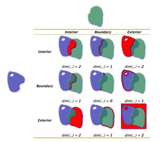
With a {T,F} matrix using the I,B, E space, there are 512 possible relations that can be grouped into binary classification schemes.
About 10 of these spatial predicates have common names such as intersects, touches, within, contains. These are the binary predicates we’ve listed in previous table.
See the Binary predicates and DE-9IM section in Spatial Data Science as well as succinct overview in slides for a previous workshop by Mike Johnson
3.3 Measures and Units
Measures (with sf) make use of the underlying GEOS library, as well as the R units library that provides measure units for R vectors. Once a coordinate reference system has been defined for features, we often want to ask questions of our data such as:
- How long is a line or a polygon perimeter (unit)
- What is the area of a polygon (unit^2)
- How far apart / close together are objects from each other (unit)
Some examples using county and gage datasets we’ve seen in previous section (with refresher again on pulling in data from a .csv file with x and y information and making it spatial):
gages <- read_csv(system.file("extdata", "Gages_flowdata.csv", package = "awra2020spatial")) |>
  dplyr::select(SOURCE_FEA, STATE, LAT_SITE, LON_SITE) |>
  st_as_sf(coords = c("LON_SITE", "LAT_SITE"), crs = 4269)
st_distance(gages[1,], gages[2,])
Units: [m]
[,1]
[1,] 58822.953.4 Spatial Subsetting
Spatial subsetting is analogous to attribute subsetting - with sf objects, we can use square bracket ([]) notation to take a spatial object and return a new object that contains only the features that relate in space to another spatial object (i.e. are within, intersect, are within distance of, are spatially disjoint, etc.).
We use the simple syntax of x[y,] to perform a spatial subset with the default operation of ‘intersects’: x[y,] is identical to x[y, , op=st_intersects]. We could also provide a different spatial predicate such as x[y, , op = st_disjoint].
Let’s run through a couple examples.
First we can demonstrate some very simple spatial subsetting examples using a particular county (polygon) in Oregon and Oregon cities (points).
or_cities <- read_sf(system.file("extdata/cities.shp", package = "Rspatialworkshop"))
mult_cnty<- aoi_get(state = "OR", county= "Multnomah") |>
  st_transform(st_crs(or_cities)) # project counties to cities
mapview(mult_cnty, alpha.regions=.07, color='black', lwd=2) + mapview(or_cities)
Spatially subset cities within Multnomah County:
3.5 Spatial Join
Often we want to join information from one spatial dataset to another based on a spatial relationship rather than attribute relationships - joining attribute data should be a familiar concept to everyone and many of the principles are the same. st_join will add new columns from from a source spatial dataset to the target spatial dataset.
By default st_join performs a left join (all rows in the target including rows with no match in the source data) - but you can also do an inner join by setting left=FALSE.
We can demonstrate the most basic spatial join using our Oregon counties and cities data - here we simply get the county name for every city based on what county each city lands in.
Rows: 898
Columns: 8
$ AREA      <dbl> 0, 0, 0, 0, 0, 0, 0, 0, 0, 0, 0, 0, 0, 0, 0, 0, 0, 0, 0, 0, …
$ PERIMETER <dbl> 0, 0, 0, 0, 0, 0, 0, 0, 0, 0, 0, 0, 0, 0, 0, 0, 0, 0, 0, 0, …
$ CITIES_   <dbl> 1, 2, 3, 4, 5, 6, 7, 8, 9, 10, 11, 12, 13, 14, 15, 16, 17, 1…
$ CITIES_ID <dbl> 1658, 1368, 1366, 1382, 1384, 1380, 1376, 1370, 1378, 1386, …
$ CITY      <chr> "MULINO", "HAMMOND", "FORT STEVENS", "GLIFTON", "BRADWOOD", …
$ FLAG      <int> 0, 0, 0, 0, 0, 0, 1, 2, 0, 0, 0, 0, 0, 0, 2, 2, 0, 0, 0, 0, …
$ geometry  <POINT [foot]> POINT (776899.8 1272019), POINT (439320.8 1638725),…
$ name      <chr> "Clackamas", "Clatsop", "Clatsop", "Clatsop", "Clatsop", "Cl…
This is equivalent to:
Rows: 898
Columns: 8
$ AREA      <dbl> 0, 0, 0, 0, 0, 0, 0, 0, 0, 0, 0, 0, 0, 0, 0, 0, 0, 0, 0, 0, …
$ PERIMETER <dbl> 0, 0, 0, 0, 0, 0, 0, 0, 0, 0, 0, 0, 0, 0, 0, 0, 0, 0, 0, 0, …
$ CITIES_   <dbl> 1, 2, 3, 4, 5, 6, 7, 8, 9, 10, 11, 12, 13, 14, 15, 16, 17, 1…
$ CITIES_ID <dbl> 1658, 1368, 1366, 1382, 1384, 1380, 1376, 1370, 1378, 1386, …
$ CITY      <chr> "MULINO", "HAMMOND", "FORT STEVENS", "GLIFTON", "BRADWOOD", …
$ FLAG      <int> 0, 0, 0, 0, 0, 0, 1, 2, 0, 0, 0, 0, 0, 0, 2, 2, 0, 0, 0, 0, …
$ geometry  <POINT [foot]> POINT (776899.8 1272019), POINT (439320.8 1638725),…
$ name <chr> "Clackamas", "Clatsop", "Clatsop", "Clatsop", "Clatsop", "Cl…3.6 Buffer and Dissolve
Typical GIS operations creating buffers around features (points, lines or polygons) and dissolving polygon boundaries based on a common attribute - here we show how to do these common GIS tasks in an R workflow.
We’ll demonstrate dissolving using both tidyverse functions in conjunction with simple features as well as using the st_union() function in sf.
Let’s use our Oregon cities and counties data again for this.
First we’ll demonstrate buffering which is a simpler operation using st_buffer with a supplied distance.
We pick our largest cities and buffer them by some arbitrary distance - we’ll say 20 miles (note below we convert feet to miles).
# Filter for metro areas
metros <- or_cities |>
  dplyr::filter(CITY %in% c('PORTLAND','SALEM','EUGENE','CORVALLIS','BEND','MEDFORD'))
# Buffer larger cities
metro_areas <- metros |>
  st_buffer(105600)
mapview(metro_areas)
Next we show both methods to dissolve, categorizing Oregon counties as urban or rural and dissolving on these categories.
# urban area
counties <- st_transform(counties, st_crs(metro_areas)) # crs same

urban_counties <- counties[metro_areas, ,op=st_intersects] # subsetting

urban <- urban_counties |>  # Dissolve
  st_union() |> # unite geometries
  st_sf() |> # promote geometry back to data frame
  dplyr::mutate(urban=TRUE) # assign urban

# rural area
# here we use tidyverse method to dissolve
rural <- counties |>
  dplyr::filter(!name %in% urban_counties$name) |>
  dplyr::group_by(state_abbr) |> # just group by state - all the same
  dplyr::mutate(AREA= geometry |> st_area()) |>
  dplyr::summarise(AREA = sum(AREA)) # this is the cool part!

mapview(urban, col.region='red') + mapview(rural)3.7 Clipping
Clipping is another extremely common GIS operation, and it’s simply a form of spatial subsetting that makes changes to the geometry list columns of affected features - it only applies to more complex geometries like lines, polygons and multi-lines and multi-polygons.
Let’s use our city buffer for Corvallis and counties to demonstrate clipping. We’ll ask for just the portions of counties that intersect our ‘metro’ buffer around Corvallis.
Let’s see what it looks like first:
plot(metro_areas[2,c('geometry')],col = "lightgrey", axes=TRUE)
plot(counties[metro_areas[2,],c('geometry')],border = "grey", add = TRUE)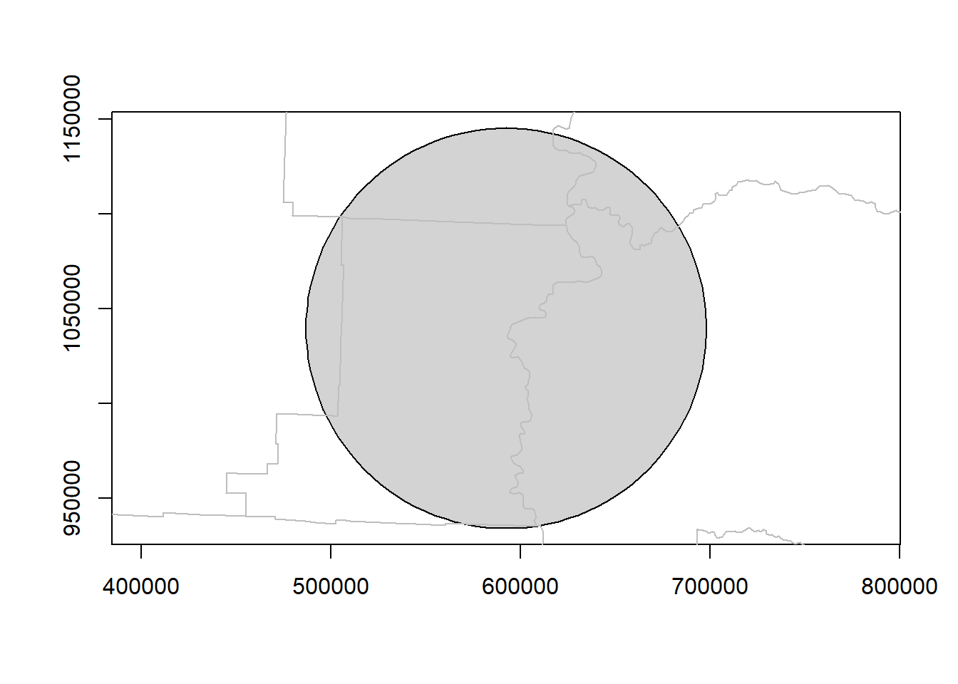
Clip and show results:
metro_county_area <- st_intersection(metro_areas[2,], counties)Warning: attribute variables are assumed to be spatially constant throughout
all geometriesplot(st_geometry(metro_county_area), border = "grey", axes = TRUE) # intersecting area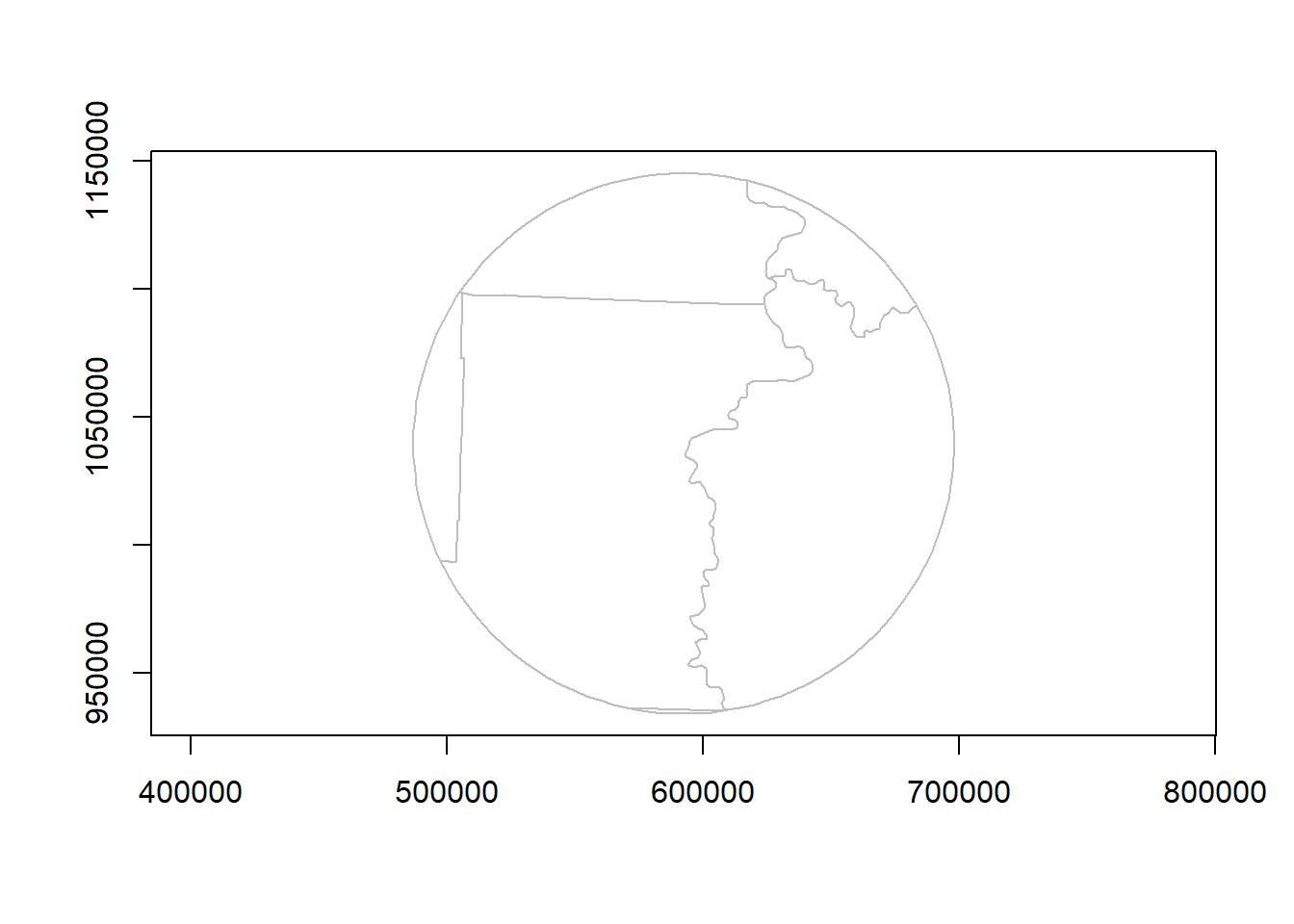
You may encounter errors like this when running geoprocessing operations like st_join in R:
Error in wk_handle.wk_wkb(wkb, s2_geography_writer(oriented
= oriented,  :  Loop 0 is not valid: Edge 772 crosses edge 774
Running st_make_valid might not fix.
You may need to turn off spherical geometry - sf_use_s2(TRUE), run st_make_valid, and then turn spherical geometry back on - sf_use_s2(FALSE) See background on S2 here and discussion of S2 related issues here
3.8 Centroids and Type Transformations
We can extract the centroid of features a couple different ways - typically we are looking for the geographic centroid which is the center of mass of a feature and can fall outside the boundaries of a feature for complex features. If we want our centroids to always be inside our features we need to ask for a point on surface. Lastly, casting in sf allows us to perform type transformations from one geometry type to another.
We’ll use our county data and bring in some river flow line data using the dataRetrieval package as well to demonstrate with linear features.
SouthSantiam <- dataRetrieval::findNLDI(nwis = "14187200", nav = "UT", find = "flowlines", distance_km=10)

SouthSantiam <- SouthSantiam$UT_flowlines
SouthSantiam <- SouthSantiam |>
  st_transform(st_crs(counties))

riv_cent1 <- st_centroid(SouthSantiam)
Warning: st_centroid assumes attributes are constant over geometriesriv_cent2 <- st_point_on_surface(SouthSantiam)Warning: st_point_on_surface assumes attributes are constant over geometriessel_counties <- counties |>
dplyr::filter(name %in% c('Marion','Yamhill','Polk','Benton','Multnomah','Clackamas','Linn','Washington'))
cnt_cent1 <- st_centroid(sel_counties)Warning: st_centroid assumes attributes are constant over geometriescnt_cent2 <- st_point_on_surface(sel_counties)Warning: st_point_on_surface assumes attributes are constant over geometriesp1 = tm_shape(sel_counties) + tm_borders() +
tm_shape(cnt_cent1) + tm_symbols(shape = 1, col = "black", size = 0.5) +
tm_shape(cnt_cent2) + tm_symbols(shape = 1, col = "red", size = 0.5)
p2 = tm_shape(SouthSantiam) + tm_lines() +
tm_shape(riv_cent1) + tm_symbols(shape = 1, col = "black", size = 0.5) +
tm_shape(riv_cent2) + tm_symbols(shape = 1, col = "red", size = 0.5)
tmap_arrange(p1, p2, ncol = 2)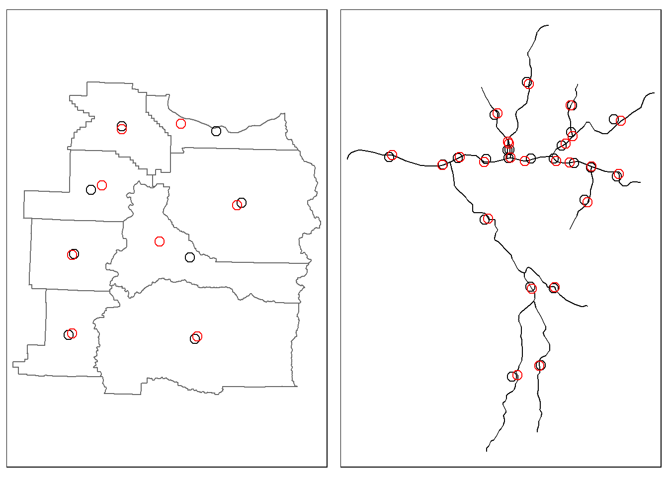
3.9 Simplification
With simplification we can generalize vector line and polygon objects - this is often useful to improve cartographic display as well as to reduce memory use and disk space used by complex geometric features. st_simplify in sf provides basic simplification implementing the Douglas-Peucker algorithm via GEOS to prune vertices. See rmapshaper and mapshaper for more extensive simplification algorithms.
Sant_simp = st_simplify(SouthSantiam, dTolerance = 500)  # 500 m
p1 = tm_shape(SouthSantiam) + tm_lines()
p2 = tm_shape(Sant_simp) + tm_lines()
tmap_arrange(p1, p2, ncol = 2)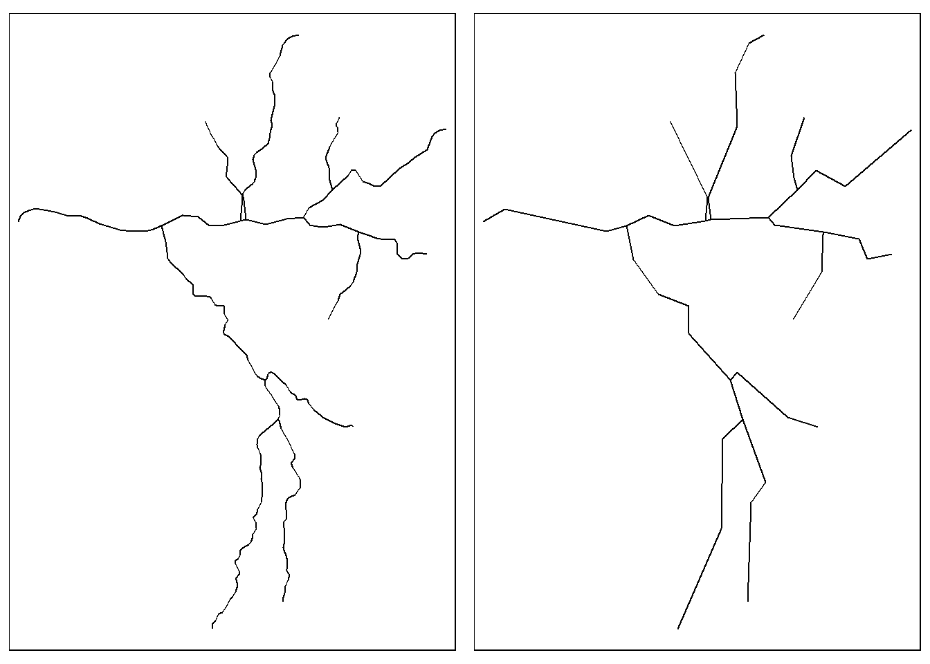
3.10 Raster operations
3.10.1 Cropping
We’ll use some built in data from a previous workshop to demonstrate a number of simple raster geoprocessing operations.
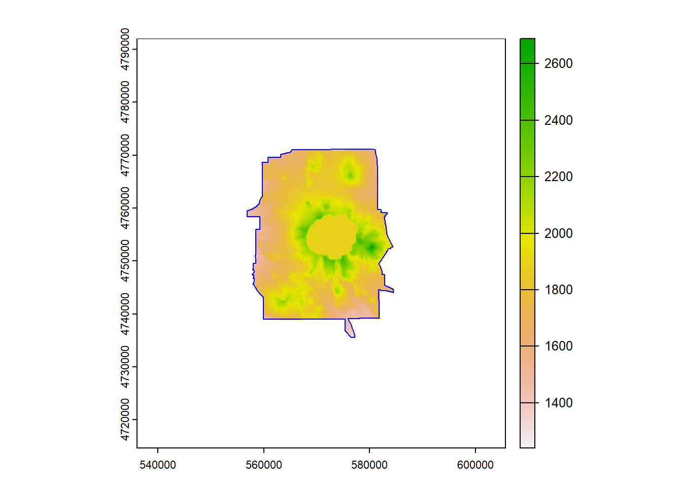
We’ll start with an elevation raster and Crater Lake boundary and project both to an local conformal projection (UTM Z10 North)
data(CraterLake)
raster_filepath <- system.file("extdata", "elevation.tif", package = "Rspatialworkshop")
elevation <- rast(raster_filepath)
elevation <- project(elevation, "EPSG:26910", method = "bilinear")
CraterLake <- st_transform(CraterLake,crs(elevation))
plot(elevation)
plot(CraterLake, add=TRUE, col=NA, border='blue')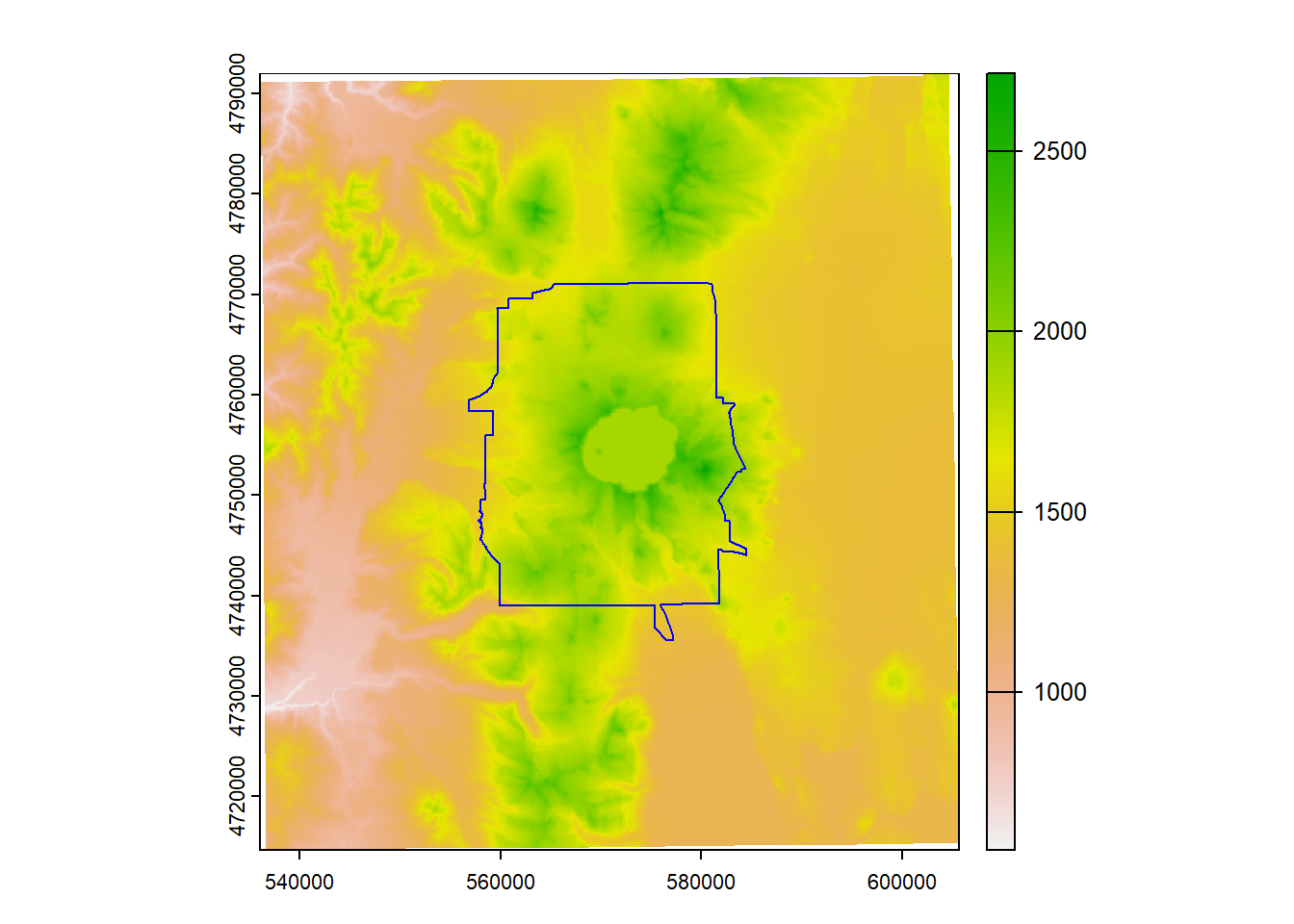
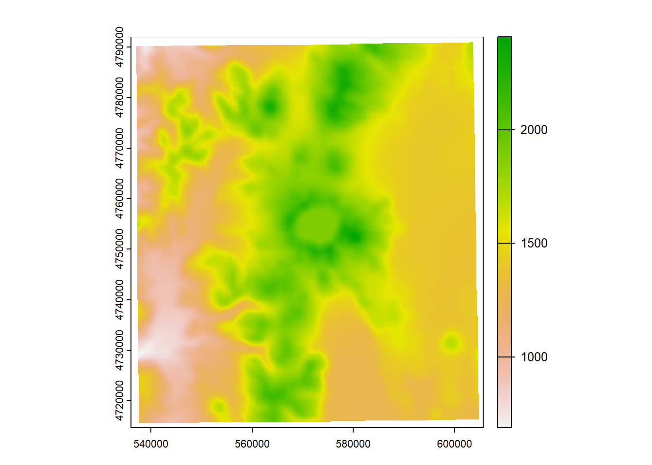
Here we’ll use crop to crop the elevation raster to the bounding box of our Crater Lake polygon feature
elev_crop = crop(elevation, vect(CraterLake))
plot(elev_crop)
plot(CraterLake, add=TRUE, col=NA, border='blue')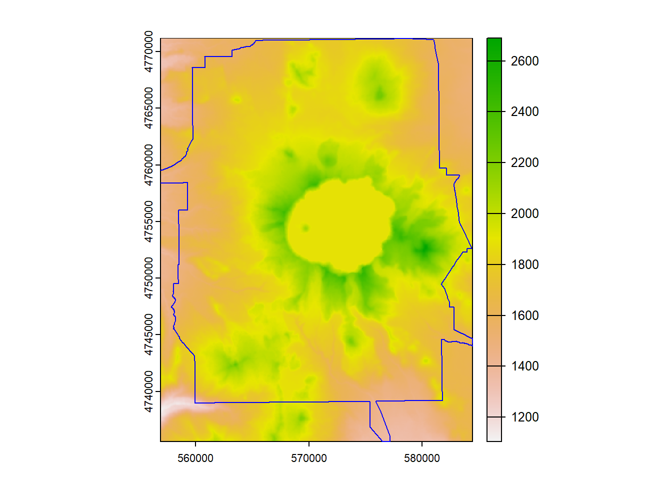
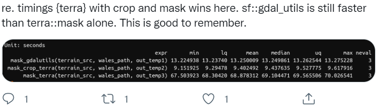
And finally we can use mask to mask the raster to just inside the polygon outline of Crater Lake National Park.
Note - if you have a large raster, it makes a HUGE difference to use crop first, then mask - mask is a much more computationally intensive operation so it will pay off to crop first then mask. An interesting twitter thread regarding this just the other day:

3.10.2 Map Algebra
We can divide map algebra into a couple of categories:
- Local - per-cell operations
- raster calculator
- replacing values
- reclassifying
- calculating indices
- Focal (neighborhood operations)
- summarizing output cell value as the result of a window (such as a3 x 3 input cell block)
- Zonal operations - summarizing raster values for some zones (either another raster or a vector feature)
- Global - summarizing values over entire raster(s)
3.10.2.1 Local Operations
Say we want to convert our elevation raster from meters to feet:
elev_feet = elevation * 3.28084
elev_feet
class : SpatRaster
dimensions : 981, 883, 1 (nrow, ncol, nlyr)
resolution : 78.76638, 78.76638 (x, y)
extent : 536109.7, 605660.4, 4714704, 4791974 (xmin, xmax, ymin, ymax)
coord. ref. : NAD83 / UTM zone 10N (EPSG:26910)
source(s) : memory
name : srtm_12_04
min value : 1846.880
max value : 8910.399 Our max value is 8890, which makes sense - the high point in Crater Lake National Park is Mount Scott at 8,929’.
What if we want to make elevation bins, or classify some elevations as NA with our elevation raster?
reclass <- matrix(c(0, 500, 1, 500, 1000, 2, 1000, 1500, 3, 1500 , 2000, 4, 2000, 2700, 5), ncol = 3, byrow = TRUE)
reclass
[,1] [,2] [,3]
[1,] 0 500 1
[2,] 500 1000 2
[3,] 1000 1500 3
[4,] 1500 2000 4
[5,] 2000 2700 5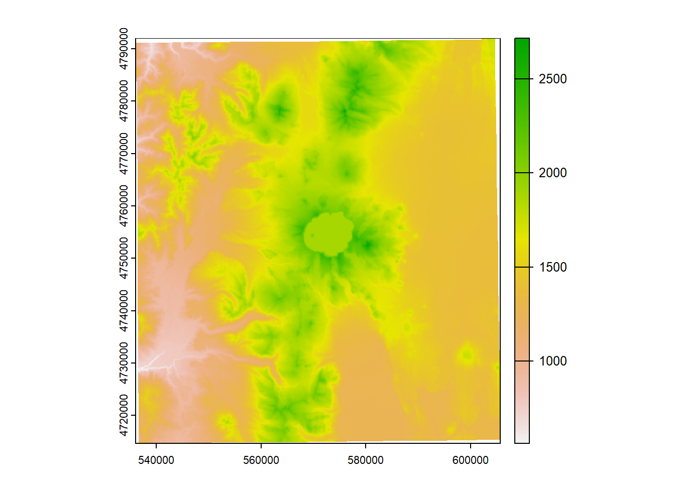
plot(elev_recl)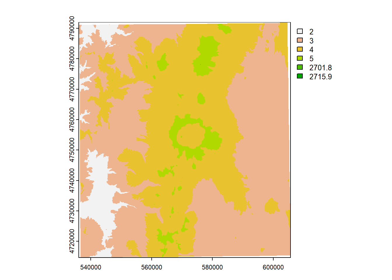
elev_new = elevation
elev_new[elev_new > 2000] = NA
plot(elev_new)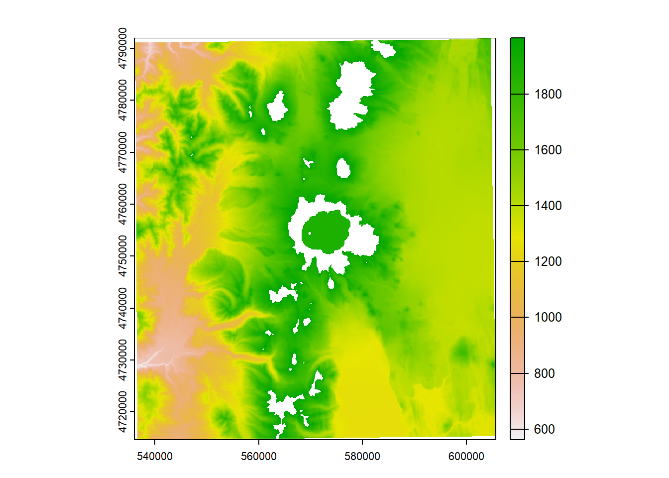
3.10.2.2 Focal Operations
A simple focal window operation
3.10.2.3 Global Operations
3.10.3 Zonal Operations
Here we demonstrate using the zonal function in terra to summarize a value raster of elevation, using an srtm.tif from spDataLarge, by the zones of NLCD classes using nlcd.tif raster also in the spDataLarge package. We’ll expand more on zonal statistics including for categorical data in the final section of the workshop.
srtm_path = system.file("raster/srtm.tif", package = "spDataLarge")
srtm_path
[1] "C:/Users/mwebe/AppData/Local/R/win-library/4.3/spDataLarge/raster/srtm.tif"srtm = rast(srtm_path)
srtmclass : SpatRaster
dimensions : 457, 465, 1 (nrow, ncol, nlyr)
resolution : 0.0008333333, 0.0008333333 (x, y)
extent : -113.2396, -112.8521, 37.13208, 37.51292 (xmin, xmax, ymin, ymax)
coord. ref. : lon/lat WGS 84 (EPSG:4326)
source : srtm.tif
name : srtm
min value : 1024
max value : 2892 nlcd = rast(system.file("raster/nlcd2011.tif", package = "spDataLarge"))
srtm_utm = project(srtm, nlcd, method = "bilinear")
srtm_zonal = zonal(srtm_utm, nlcd, na.rm = TRUE, fun = "mean")
srtm_zonal nlcd2011 srtm
1 11 2227.060
2 21 1713.980
3 22 1642.077
4 23 1569.632
5 31 1854.069
6 41 2361.121
7 42 1867.068
8 43 2500.253
9 52 1650.966
10 71 1644.359
11 81 1284.106
12 82 1417.671
13 90 1254.168
14 95 1909.590