1 Foundations

1.1 Goals and Outcomes

Understand fundamental spatial data structures and libraries in R.
Become familiar with coordinate reference systems.
Geographic I/O (input/output)

Throughout this section we’ll use the following packages:

library(dataRetrieval)
library(tmap)
library(tmaptools)
library(dplyr)
library(tigris)
library(sf)
library(mapview)
mapviewOptions(fgb=FALSE)
library(ggplot2)
library(spData)
library(terra)
library(stars)
library(Rspatialworkshop)
library(readr)
library(cowplot)
library(knitr)
library(dplyr)
library(rnaturalearth)
library(osmdata)
library(terra)
library(stars)

1.2 Background on data structures

Note

Much of this background on data structures is borrowed from Mike Johnson’s Introduction to Spatial Data Science and lecture material from our AWRA 2022 Geo Workshop

Before we dive into spatial libraries, it’s worth a quick review of relevant data structures in R - this will be a whirlwind overview, assuming most everyone is familiar with using R already.

You, computers, and software ‘understand’ values in particular and different ways
Computers convert bytes –> hex –> value
- Humans read values
- Software reads Hex bytes
- Hardware reads Binary bytes

Note

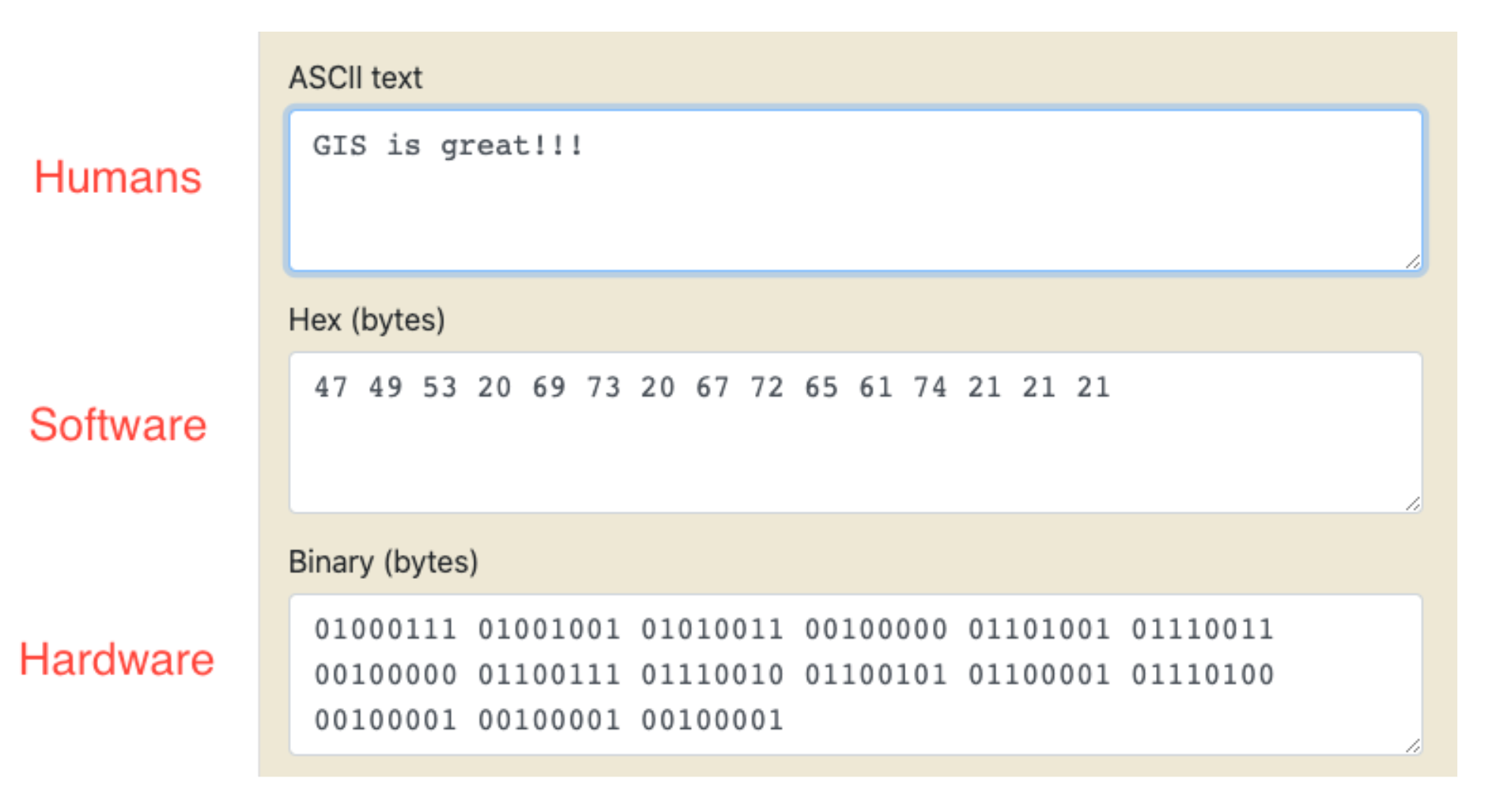
What’s the difference between 10 and ‘10’?

To us: meaning
To software: how it is handled
To a computer: nothing

We need human-defined (computer-guessable) data types

Fundamental data types

# Numeric
typeof(1.9)
#> [1] "double"
# Integer
typeof(1L)
#> [1] "integer"
# Boolean
typeof(TRUE)
#> [1] "logical"
# Character
typeof("Welcome")
#> [1] "character"

Storing more than one value requires a structure.

Values can be structured in ways such as:

vectors
dimensions/attributes
data.frames

And data.frames can be operated on with functions such as:

filter
select
mutate
summarize
group_by

1.2.1 Vectors

Note

‘vector’ has two meanings when working with GIS data and working in R!

geographic vector data (which we’ll explore)
vector class (what we’re talking about here)

geographic vector data is a data model, and the vector class is an R class like data.frame and matrix

Vectors come in two flavors:

atomic
list

atomic vectors elements must have the same type
lists elements can have different types

1.2.2 Atomic vectors

# Numeric
dbl_vec = c(1.9, 2, 3.5)
typeof(dbl_vec)
#> [1] "double"
length(dbl_vec)
#> [1] 3
# Logical
lg_vec = c(TRUE, FALSE, F, T)
typeof(lg_vec)
#> [1] "logical"
length(lg_vec)
#> [1] 4

Coercion

type is a property of a vector
When you try to combine different types they’ll be coerced in the following fixed order:
- character => double => integer => logical
Coercion occurs automatically but generates a warning and a missing value when it fails

c("a", 1)
#> [1] "a" "1"
c("a", TRUE)
#> [1] "a"    "TRUE"
c(4.5, 1L)
#> [1] 4.5 1.0
c("1", 18, "GIS")
#> [1] "1"   "18"  "GIS"
as.numeric(c("1", 18, "GIS"))
#> [1]  1 18 NA
as.logical(c("1", 18, "GIS"))
#> [1] NA NA NA

Subsetting atomic vectors

# Atomic numeric vector
(x = c(3.4, 7, 18, 9.6))
#> [1]  3.4  7.0 18.0  9.6

# Third Value
x[3]
#> [1] 18

# Third and Fourth value
x[c(3,4)]
#> [1] 18.0  9.6

# Drop the third value
x[-3]
#> [1] 3.4 7.0 9.6

# Keep the 1 and 2 value, but drop 3 and 4
x[c(T,T,F,F)]
#> [1] 3.4 7.0

1.2.3 Matrix

A matrix is 2D atomic (row, column)
- Same data types
- Same column length

This is how spatial raster data is structured

Subsetting matrices uses row,column (i,j) syntax

(x = matrix(1:9, nrow = 3))
#>      [,1] [,2] [,3]
#> [1,]    1    4    7
#> [2,]    2    5    8
#> [3,]    3    6    9
x[3,]
#> [1] 3 6 9
x[,3]
#> [1] 7 8 9
x[3,3]
#> [1] 9

1.2.4 Array

Array is a 3d Atomic (row, column, slice)

This is how spatial raster data with a time dimension is structured

(array(c(1:12), dim = c(3,2,2)))
#> , , 1
#> 
#>      [,1] [,2]
#> [1,]    1    4
#> [2,]    2    5
#> [3,]    3    6
#> 
#> , , 2
#> 
#>      [,1] [,2]
#> [1,]    7   10
#> [2,]    8   11
#> [3,]    9   12

Subsetting arrays uses row, column, slice syntax (i,j,z)

(x = array(1:12, dim = c(2,2,3)))
#> , , 1
#> 
#>      [,1] [,2]
#> [1,]    1    3
#> [2,]    2    4
#> 
#> , , 2
#> 
#>      [,1] [,2]
#> [1,]    5    7
#> [2,]    6    8
#> 
#> , , 3
#> 
#>      [,1] [,2]
#> [1,]    9   11
#> [2,]   10   12
x[1,,]
#>      [,1] [,2] [,3]
#> [1,]    1    5    9
#> [2,]    3    7   11
x[,1,]
#>      [,1] [,2] [,3]
#> [1,]    1    5    9
#> [2,]    2    6   10
x[,,1]
#>      [,1] [,2]
#> [1,]    1    3
#> [2,]    2    4

1.2.5 Lists

Eash list element can be any data type

(my_list <- list(
  matrix(1:4, nrow = 2), 
  "GIS is great!", 
  c(TRUE, FALSE, TRUE), 
  c(2.3, 5.9)
))
#> [[1]]
#>      [,1] [,2]
#> [1,]    1    3
#> [2,]    2    4
#> 
#> [[2]]
#> [1] "GIS is great!"
#> 
#> [[3]]
#> [1]  TRUE FALSE  TRUE
#> 
#> [[4]]
#> [1] 2.3 5.9

typeof(my_list)
#> [1] "list"

Subsetting Lists

Each element of a list can be accessed with the [[ operator

my_list[[1]]
#>      [,1] [,2]
#> [1,]    1    3
#> [2,]    2    4
my_list[[1]][1,2]
#> [1] 3

1.2.6 Data Frames

data.frame is built on the list structure in R
length of each atomic or list vector has to be the same
This gives data.frame objects rectangular structure so they share properties of both matrices and lists

(df1 <- data.frame(name = c("Me", "Tim", "Sarah"),
                  age  = c(53,15,80),
                  retired = c(F,F,T)))
#>    name age retired
#> 1    Me  53   FALSE
#> 2   Tim  15   FALSE
#> 3 Sarah  80    TRUE
typeof(df1)
#> [1] "list"

Subsetting a data.frame

df1[1,2]
#> [1] 53

# or like a list
df1[[2]]
#> [1] 53 15 80

# or with column name operator
df1$name
#> [1] "Me"    "Tim"   "Sarah"

1.2.7 Data manipulation

data.frame manipulation is all based on SQL queries
R abstracts the SQL logic and provides function-ized methods
dplyr in the tidyverse ecosystem provides the ’grammar of data manipulation` approach we’ll use in this workshop

Data manipulation verbs:

Primary:
- select(): keeps or removes variables based on names
- filter(): keeps or removes observations based on values _ Manipulation:
- mutate(): adds new variables that are functions of existing variables
- summarise(): reduces multiple values down to a single summary
- arrange(): changes ordering of the rows
Grouping:
- group_by(): combine with any or all of the above to perform manipulation ‘by group’

1.2.8 Pipe operator

The pipe operator (native R pipe operator |> or magrittr pipe operator %>%) provides a more concise and expressive coding experience
The pipe passes the object on the left hand side of the pipe into the first argument of the right hand function
To be |> compatible, the data.frame is ALWAYS the fist argument to dplyr verbs

A demonstration using dataRetrieval package stream gage data from USGS:

flows <- dataRetrieval::readNWISdv(
  siteNumbers = '14187200',
  parameterCd = "00060"
)  |>  
  dataRetrieval::renameNWISColumns()
  
dplyr::glimpse(flows)
#> Rows: 18,340
#> Columns: 5
#> $ agency_cd <chr> "USGS", "USGS", "USGS", "USGS", "USGS", "USGS", "USGS", "…
#> $ site_no   <chr> "14187200", "14187200", "14187200", "14187200", "14187200…
#> $ Date      <date> 1973-08-01, 1973-08-02, 1973-08-03, 1973-08-04, 1973-08-…
#> $ Flow      <dbl> 809, 828, 829, 930, 939, 939, 944, 932, 927, 925, 927, 92…
#> $ Flow_cd   <chr> "A", "A", "A", "A", "A", "A", "A", "A", "A", "A", "A", "A…

Exercise

What is the :: after the package name and before the function in the R code above doing? How would you find out more about it?

Solution

:: specifies the namespace (i.e., package) associated with a particular function.

You can get help on it the same way you get help on anything in R:

?'::'
# or
help("::")

1.2.9 Filter

filter() takes logical (binary) expressions and returns the rows in which all conditions are TRUE.

Filter on a single condition:

flows |> 
  dplyr::filter(Flow > 900) |>
  dplyr::glimpse()
#> Rows: 14,449
#> Columns: 5
#> $ agency_cd <chr> "USGS", "USGS", "USGS", "USGS", "USGS", "USGS", "USGS", "…
#> $ site_no   <chr> "14187200", "14187200", "14187200", "14187200", "14187200…
#> $ Date      <date> 1973-08-04, 1973-08-05, 1973-08-06, 1973-08-07, 1973-08-…
#> $ Flow      <dbl> 930, 939, 939, 944, 932, 927, 925, 927, 928, 945, 938, 94…
#> $ Flow_cd   <chr> "A", "A", "A", "A", "A", "A", "A", "A", "A", "A", "A", "A…

Or multiple conditions:

flows  |> 
  dplyr::filter(Flow > 900, Date > as.Date("2010-01-01"))  |>
  dplyr::glimpse()
#> Rows: 4,399
#> Columns: 5
#> $ agency_cd <chr> "USGS", "USGS", "USGS", "USGS", "USGS", "USGS", "USGS", "…
#> $ site_no   <chr> "14187200", "14187200", "14187200", "14187200", "14187200…
#> $ Date      <date> 2010-01-02, 2010-01-03, 2010-01-04, 2010-01-05, 2010-01-…
#> $ Flow      <dbl> 7870, 6920, 5860, 7860, 10000, 10100, 9760, 9130, 8600, 7…
#> $ Flow_cd   <chr> "A", "A", "A", "A", "A", "A", "A", "A", "A", "A", "A", "A…

1.2.10 Select

Subset variables (columns) you want to keep or exclude by name

Just keep three columns

flows |> 
  dplyr::select(Date, Flow)  |> 
  dplyr::glimpse()
#> Rows: 18,340
#> Columns: 2
#> $ Date <date> 1973-08-01, 1973-08-02, 1973-08-03, 1973-08-04, 1973-08-05, 1…
#> $ Flow <dbl> 809, 828, 829, 930, 939, 939, 944, 932, 927, 925, 927, 928, 94…

Exclude just one

flows |> 
  dplyr::select(-Flow_cd)  |> 
  dplyr::glimpse()
#> Rows: 18,340
#> Columns: 4
#> $ agency_cd <chr> "USGS", "USGS", "USGS", "USGS", "USGS", "USGS", "USGS", "…
#> $ site_no   <chr> "14187200", "14187200", "14187200", "14187200", "14187200…
#> $ Date      <date> 1973-08-01, 1973-08-02, 1973-08-03, 1973-08-04, 1973-08-…
#> $ Flow      <dbl> 809, 828, 829, 930, 939, 939, 944, 932, 927, 925, 927, 92…

..And can rename while selecting

flows |> 
  dplyr::select(Date, flow_cfs = Flow)  |> 
  dplyr::glimpse()
#> Rows: 18,340
#> Columns: 2
#> $ Date     <date> 1973-08-01, 1973-08-02, 1973-08-03, 1973-08-04, 1973-08-0…
#> $ flow_cfs <dbl> 809, 828, 829, 930, 939, 939, 944, 932, 927, 925, 927, 928…

1.2.11 Mutate

mutate() defines and inserts new variables into a existing data.frame
mutate() builds new variables sequentially so you can reference earlier ones when defining later ones

We can extract Year and Month as new variables from the Date variable using date time

flows  |> 
  dplyr::select(Date, Flow)  |>  
  dplyr::filter(Date > as.Date('2010-01-01'))  |> 
  dplyr::mutate(Year  = format(Date, "%Y"), Month = format(Date, "%m"))  |>  
  dplyr::glimpse()
#> Rows: 5,037
#> Columns: 4
#> $ Date  <date> 2010-01-02, 2010-01-03, 2010-01-04, 2010-01-05, 2010-01-06, …
#> $ Flow  <dbl> 7870, 6920, 5860, 7860, 10000, 10100, 9760, 9130, 8600, 7040,…
#> $ Year  <chr> "2010", "2010", "2010", "2010", "2010", "2010", "2010", "2010…
#> $ Month <chr> "01", "01", "01", "01", "01", "01", "01", "01", "01", "01", "…

1.2.12 Summarize and Group_By

summarize() allows you to summarize across all observations
group_by() allows you to apply any of these manipulation verbs by group in your data

flows |> 
 dplyr::select(Date, Flow) |> 
 dplyr::mutate(Year  = format(Date, "%Y"))  |> 
 dplyr::group_by(Year) |> 
 dplyr::summarize(meanQ = mean(Flow),
           maxQ = max(Flow))
#> # A tibble: 51 × 3
#>    Year  meanQ  maxQ
#>    <chr> <dbl> <dbl>
#>  1 1973  4669. 13200
#>  2 1974  3659. 14400
#>  3 1975  3611. 14100
#>  4 1976  2340. 15000
#>  5 1977  2860. 16200
#>  6 1978  2206. 11300
#>  7 1979  2378. 12000
#>  8 1980  2548. 14700
#>  9 1981  2976. 17000
#> 10 1982  3424. 15100
#> # ℹ 41 more rows

Note

You may click on any of the functions in this book to be directed to their respective documentation. For example, clicking on st_join() takes you to the documentation page for the st_join() function on the sf website.

1.3 Why R for Spatial Data Analysis?

Advantages

R is:
- lightweight
- open-source
- cross-platform
Works with contributed packages - currently 19883
- provides extensibility
Automation and recording of workflow
provides reproducibility
Optimized work flow - data manipulation, analysis and visualization all in one place
- provides integration
R does not alter underlying data - manipulation and visualization in memory
R is great for repetitive graphics
R is great for integrating different aspects of analysis - spatial and statistical analysis in one environment
- again, integration
Leverage statistical power of R (i.e. modeling spatial data, data visualization, statistical exploration)
Can handle vector and raster data, as well as work with spatial databases and pretty much any data format spatial data comes in
R’s GIS capabilities growing rapidly right now - new packages added monthly - currently about 275 spatial packages (depending on how you categorize)

Drawbacks for usig R for GIS work

R is not as good for interactive use as desktop GIS applications like ArcGIS or QGIS (i.e. editing features, panning, zooming, and analysis on selected subsets of features)
Explicit coordinate system handling by the user
- no on-the-fly projection support
In memory analysis does not scale well with large GIS vector and tabular data
Steep learning curve
Up to you to find packages to do what you need - help not always great

1.3.1 A Couple Motivating Examples

Here’s a quick example demonstrating R’s flexibility and current strength for plotting and interactive mapping with very simple, expressive code:

# find my town!
my_town <-tmaptools::geocode_OSM("Corvallis OR USA", as.sf = TRUE)
glimpse(my_town)
#> Rows: 1
#> Columns: 9
#> $ query   <chr> "Corvallis OR USA"
#> $ lat     <dbl> 44.56457
#> $ lon     <dbl> -123.262
#> $ lat_min <dbl> 44.51993
#> $ lat_max <dbl> 44.60724
#> $ lon_min <dbl> -123.3362
#> $ lon_max <dbl> -123.231
#> $ bbox    <POLYGON [°]> POLYGON ((-123.3362 44.5199...
#> $ point   <POINT [°]> POINT (-123.262 44.56457)

Exercise

Run and examine code chunk above and try geocoding examples you think of

What does :: do?
What does geocode_OSM() do?
Explain how the code runs together using the |> chaining operator
What is glimpse()? How is it useful compared to head()?

Solution

:: specifies using geocode_OSM from the tmaptools package. R gives namespace preference to packages in order loaded. Some packages share function names, so when there is ambiguity, it’s good practice to disambiguate your functions with the double-colon
geocode_OSM() looks up a named features in OpenStreetMap and returns the coordinates (bonus - we’ll delve into more in next section - what coordinate reference system are coordinates in and how do you find out?)
You would translate code using the |> operator from:

do this |> do that |> do that

do this then do that then do that

Technically, it’s a transposed version of print() - columns run down page, data across like rows - it additionally gives you the number of observations and variables, and the data type of each column. Note that glimpse() omits geometry information - you would type the name of your object at the console to get full information, or use print.sf() or str().

bonus: how would you quickly learn more about glimpse() from the console?

1.3.1.1 Choropleth map

The tigris package can be used to get census boundaries such as states and counties as vector sf objects in R

counties <- counties("Oregon", cb = TRUE)
counties$area <- as.numeric(st_area(counties))
glimpse(counties)

tm_shape(counties) +
  tm_polygons("area", style="quantile", title="Area of Oregon Counties")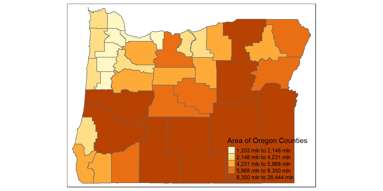

1.3.1.2 Interactive mapping

mapview(my_town, col="red", col.regions = "red") +
  mapview(counties, alpha.regions = .1)

1.4 Spatial Data Structures in R

First we’ll walk through spatial data structures in R and review some key components of data structures in R that inform our use of spatial data in R.

Note

A few core libraries underpin spatial libraries in R (and Python!) and in GIS software applications such as QGIS and ArcPro. Spatial data structures across languages and applications are primarily organized through OSgeo and OGC). These core libraries include:

GDAL –> For raster and feature abstraction and processing
PROJ –> A library for coordinate transformations and projections
GEOS –> A Planar geometry engine for operations (measures, relations) such as calculating buffers and centroids on data with a projected CRS
S2 –> a spherical geometry engine written in C++ developed by Google and adapted in R with the s2 package

We’ll see how these core libraries are called and used in the R packages we explore throughout this workshop.

Note

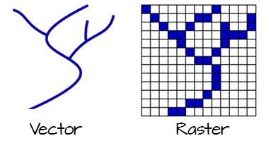
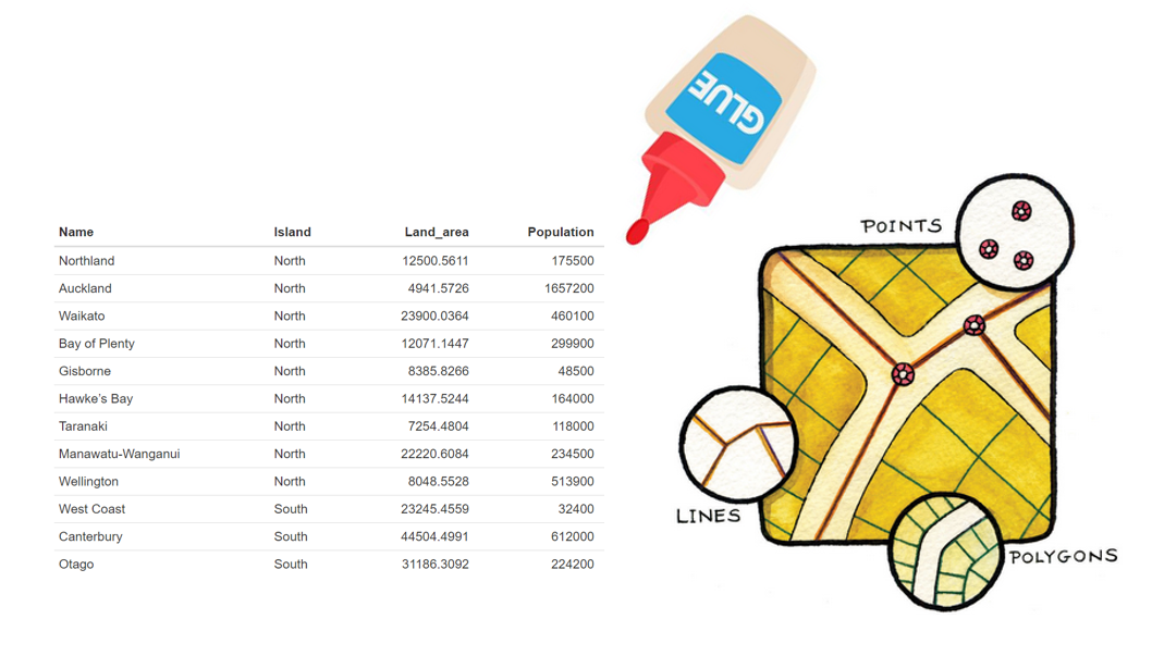
Vector data are comprised of points, lines, and polygons that represent discrete spatial entities, such as a river, watershed, or stream gauge.
Raster data divides spaces into rectilinear cells (pixels) to represent spatially continuous phenomena, such as elevation or the weather. The cell size (or resolution) defines the fidelity of the data.

1.4.1 Vector Data Model

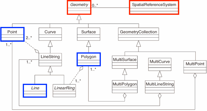
For Vector data, Simple Features (officially Simple Feature Access) is both an OGC and International Organization for Standardization (ISO) standard that specifies how (mostly) two-dimensional geometries can represent and describe objects in the real world. The Simple Features specification includes:

a class hierarchy
a set of operations
binary and text encodings

It describes how such objects can be stored in and retrieved from databases, and which geometrical operations should be defined for them.

It outlines how the spatial elements of POINTS (XY locations with a specific coordinate reference system) extend to LINES, POLYGONS and GEOMETRYCOLLECTION(s).

The “simple” adjective also refers to the fact that the line or polygon geometries are represented by sequences of points connected with straight lines that do not self-intersect.

Figure 1.2: The simple features data model.

Here we’ll load the sf library to load the classes and functions for working with spatial vector data and to explore how sf handles vector spatial data in R:

library(sf)

Question

What is the message you see in your console the first time you load sf? Hint: If you don’t see a message, you probably already have the sf library attached - you can uncheck it in your packages pane in RStudio, or you can run detach("package:sf", unload = TRUE)

Answer

The output from library(sf) reports which versions of key geographic libraries such as GEOS the package is using

You can report on versions of external software used by sf with:

sf::sf_extSoftVersion()
#>           GEOS           GDAL         proj.4 GDAL_with_GEOS     USE_PROJ_H 
#>        "3.9.3"        "3.5.2"        "8.2.1"         "true"         "true" 
#>           PROJ 
#>        "8.2.1"

We’ll cover highlights of the functionality of sf but we encourage you to read the sf package website documentation r-spatial.github.io/sf which can be viewed offline in RStudio using:

vignette(package = "sf") # see which vignettes are available
vignette("sf1")          # open the introduction vignette

The sfg class in sf represents the different simple feature geometry types in R: point, linestring, polygon (and ‘multi’ equivalents such as multipoints) or geometry collection. Vector data in R and sf can be broken down into three basic geometric primitives with equivalent sf functions to create them:

points - st_points()
linestrings - st_linestring()
polygons - st_polygon()

We buld up the more complex simple feature geometries with: - st_multipoint() for multipoints - st_multilinestring() for multilinestrings - st_multipolygon() for multipolygons - st_geometrycollection() for geometry collections

Typically we don’t build these up from scratch ourselves but it’s important to understand these building blocks since primitives are the building blocks for all vector features in sf

All functions and methods in sf that operate on spatial data are prefixed by st_, which refers to spatial type.
This is similar to PostGIS
This makes them sf functions easily discoverable by command-line completion.
Simple features are also native R data, using simple data structures (S3 classes, lists, matrix, vector).

These primitives can all be broken down into set(s) of numeric x,y coordinates with a known coordinate reference system (crs).

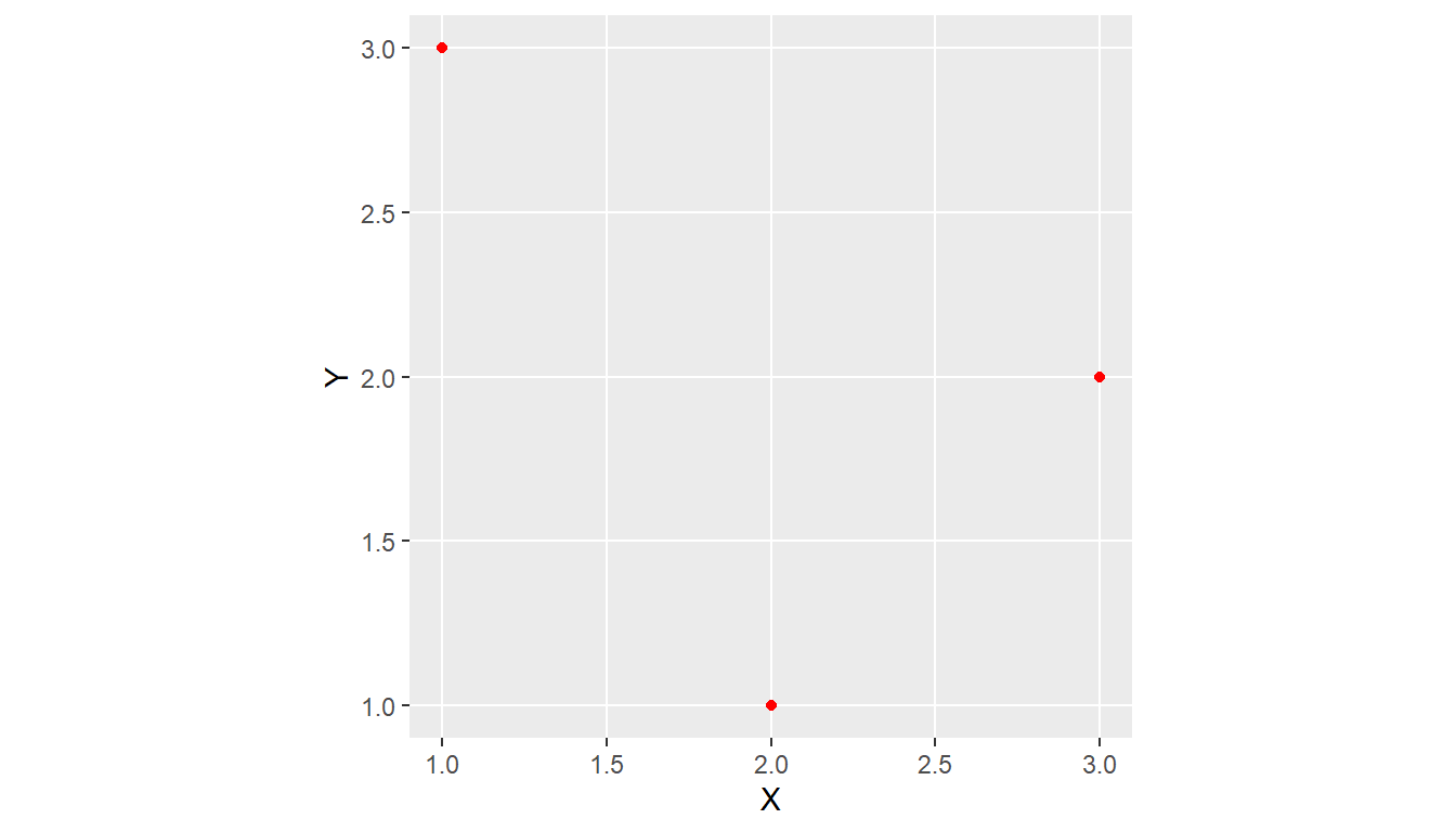
1.4.1.1 Points

A point in sf is composed of one coordinate pair (XY) in a specific coordinate system.
A POINT has no length, no area and a dimension of 0.
z and m coordinates As well as having the necessary X and Y coordinates, single point (vertex) simple features can have:
a Z coordinate, denoting altitude, and/or
an M value, denoting some “measure”

# create sf object as point
pt1 <- st_point(c(1,3))
pt2 <- st_point(c(2,1))
pt3 <- st_point(c(3,2))
sf_point <- st_sfc(pt1, pt2, pt3)

# POINT defined as numeric vector
(sf::st_dimension(sf_point))
#> [1] 0 0 0

ggplot(sf_point) + 
  geom_sf(color = "red") +
  labs(x = "X", y = "Y")

1.4.1.2 Lines

A polyline is composed of an ordered sequence of two or more POINTs
Points in a line are called vertices/nodes and explicitly define the connection between two points.
A LINESTRING has a length, has no area and has a dimension of 1 (length)

# create sf object as linestring
line1 <- sf::st_linestring(rbind(pt1, pt2))
line2 <- sf::st_linestring(rbind(pt2, pt3))
sf_linestring <- st_sfc(line1, line2)

# dimension
(sf::st_dimension(sf_linestring))
#> [1] 1 1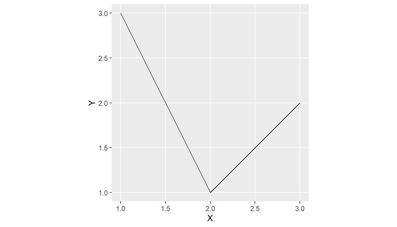

ggplot(sf_linestring) + 
  geom_sf() +
  labs(x = "X", y = "Y")

1.4.1.3 Polygon

A POLYGON is composed of 4 or more points whose starting and ending point are the same.
A POLYGON is a surface stored as a list of its exterior and interior rings.
A POLYGON has length, area, and a dimension of 2. (area)

pt4 <- pt1
poly1 <- st_polygon(list(rbind(pt1, pt2, pt3, pt4)))
sf_polygon <- st_sfc(poly1)

# dimension
sf::st_dimension(sf_polygon)
#> [1] 2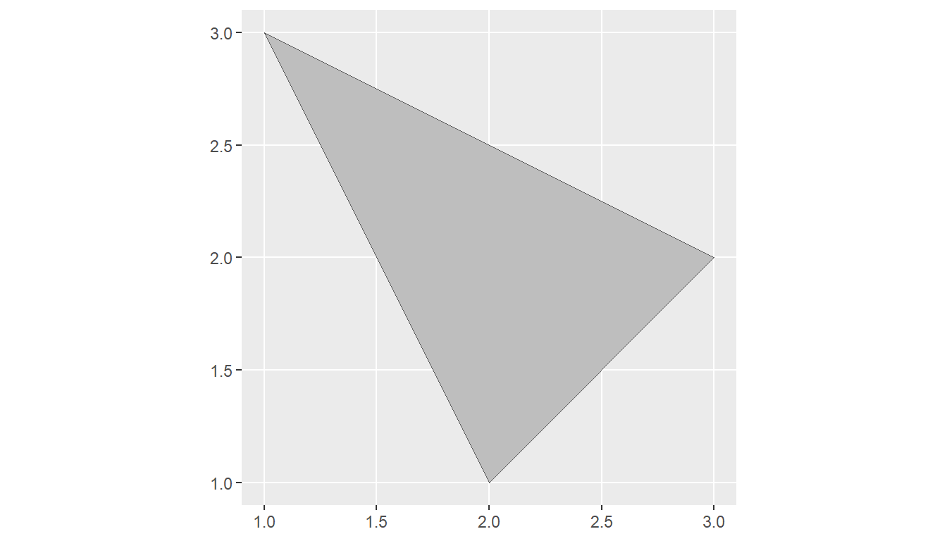

ggplot(sf_polygon) + 
  geom_sf(fill = "grey")

These geometries as we created above are structure using the WKT format. sf usesWKTandWKB` formats to store vector geometry.

1.4.1.4 Points, Lines, Polygons

We visualize all geometries together by running

ggplot() +
  geom_sf(data = sf_point, color = "red") +
  geom_sf(data = sf_linestring) +
  geom_sf(data = sf_polygon, fill = "grey")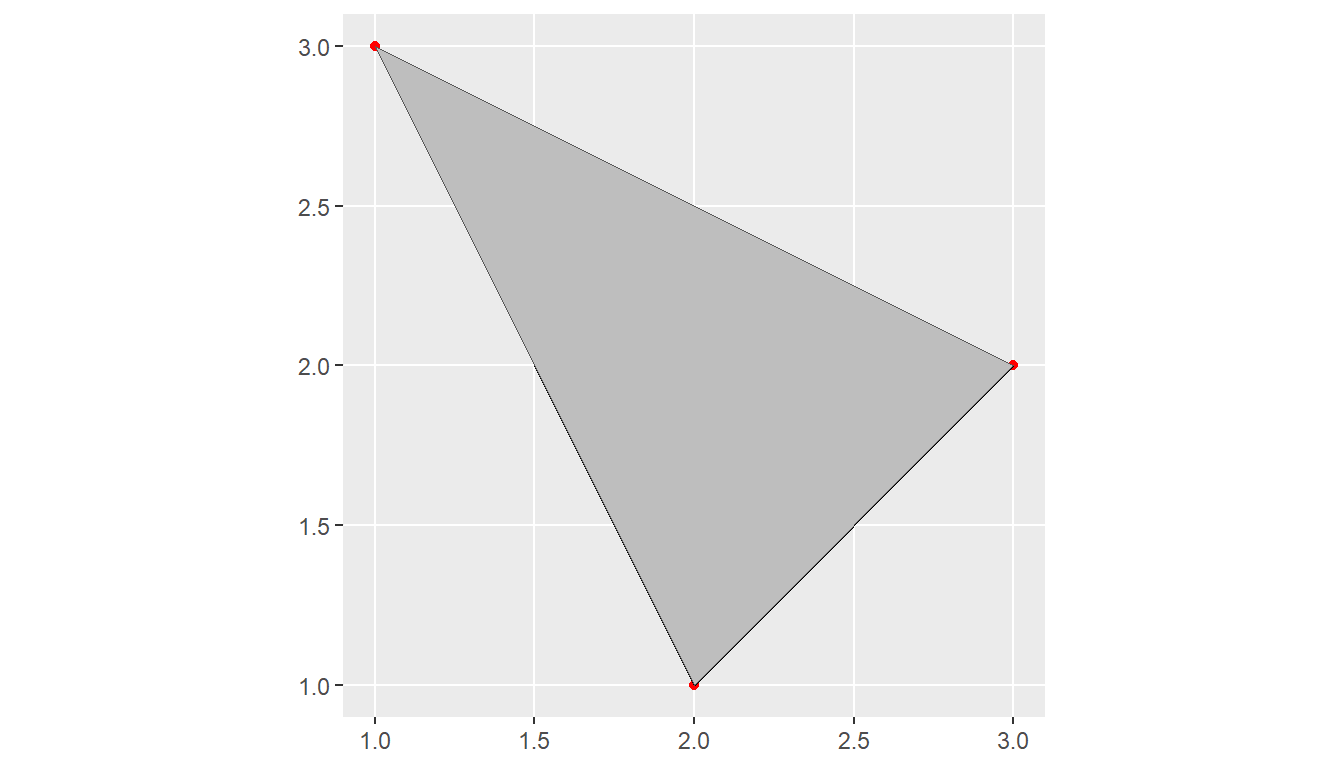

Note

WKT (Well-Known Text) and WKB

-Well-known text (WKT) encoding provide a human-readable description of the geometry. - The well-known binary (WKB) encoding is machine-readable, lossless, and faster to work with than text encoding.

WKB is used for all interactions with GDAL and GEOS.

1.4.1.5 Spatial Data Frames

Building up from basic points, lines and strings, simple feature objects are stored in a data.frame, with geometry data in a special list-column, usually named ‘geom’ or ‘geometry’ - this is the same convention used in the popular Python package GeoPandas.

Let’s look at an example spatial data set that comes in the spData package, us_states:

data("us_states")
class(us_states)
#> [1] "sf"         "data.frame"
names(us_states)
#> [1] "GEOID"        "NAME"         "REGION"       "AREA"        
#> [5] "total_pop_10" "total_pop_15" "geometry"

We see that it’s an sf data frame with both attribute columns and the special geometry column we mentioned earlier - in this case named geometry.

us_states$geometry is the ‘list column’ that contains the all the coordinate information for the US state polygons in this dataset.

To reiterate, us_states is an sf simple feature collection which we can verify with:

us_states
#> Simple feature collection with 49 features and 6 fields
#> Geometry type: MULTIPOLYGON
#> Dimension:     XY
#> Bounding box:  xmin: -124.7042 ymin: 24.55868 xmax: -66.9824 ymax: 49.38436
#> Geodetic CRS:  NAD83
#> First 10 features:
#>    GEOID        NAME   REGION             AREA total_pop_10 total_pop_15
#> 1     01     Alabama    South 133709.27 [km^2]      4712651      4830620
#> 2     04     Arizona     West 295281.25 [km^2]      6246816      6641928
#> 3     08    Colorado     West 269573.06 [km^2]      4887061      5278906
#> 4     09 Connecticut Norteast  12976.59 [km^2]      3545837      3593222
#> 5     12     Florida    South 151052.01 [km^2]     18511620     19645772
#> 6     13     Georgia    South 152725.21 [km^2]      9468815     10006693
#> 7     16       Idaho     West 216512.66 [km^2]      1526797      1616547
#> 8     18     Indiana  Midwest  93648.40 [km^2]      6417398      6568645
#> 9     20      Kansas  Midwest 213037.08 [km^2]      2809329      2892987
#> 10    22   Louisiana    South 122345.76 [km^2]      4429940      4625253
#>                          geometry
#> 1  MULTIPOLYGON (((-88.20006 3...
#> 2  MULTIPOLYGON (((-114.7196 3...
#> 3  MULTIPOLYGON (((-109.0501 4...
#> 4  MULTIPOLYGON (((-73.48731 4...
#> 5  MULTIPOLYGON (((-81.81169 2...
#> 6  MULTIPOLYGON (((-85.60516 3...
#> 7  MULTIPOLYGON (((-116.916 45...
#> 8  MULTIPOLYGON (((-87.52404 4...
#> 9  MULTIPOLYGON (((-102.0517 4...
#> 10 MULTIPOLYGON (((-92.01783 2...

We see information on

the geometry type
the dimensionality
the bounding box
the coordinate reference system
the header of the attributes

Remember that sf simple feature collections are composed of:

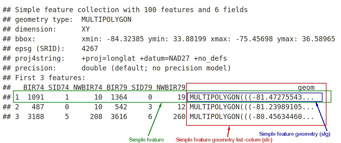
rows of simple features (sf) that contain attributes and geometry - in green
each of which have a simple feature geometry list-column (sfc) - in red
which contains the underlying simple feature geometry (sfg) for each simple feature - in blue

sf extends the generic plot function so that plot will naturally work with sf objects.

plot(us_states)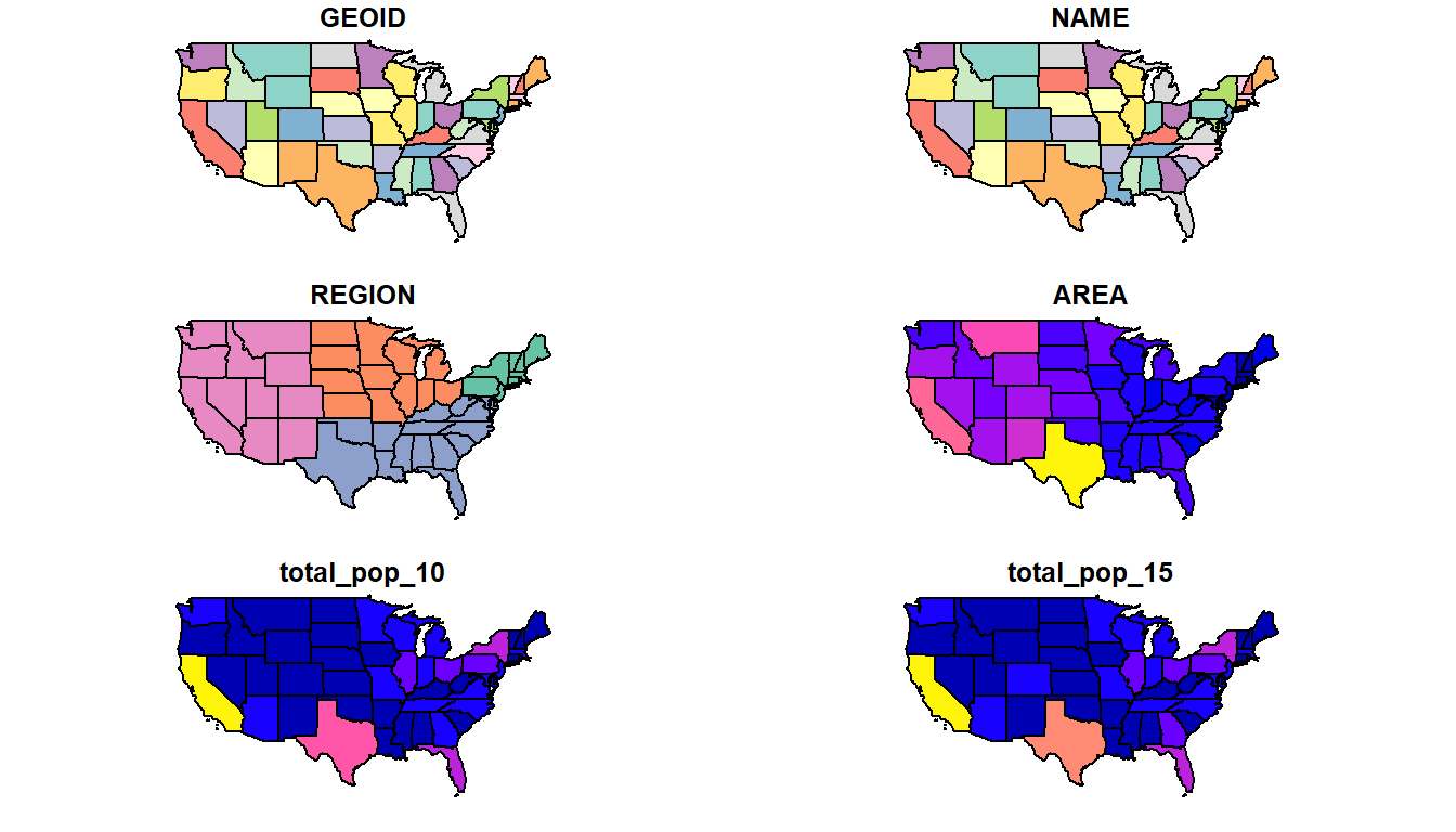

Exercise

Is this the result you expected from plot()?

Instead of making a single default map of your geometry, plot() in sf maps each variable in the dataset.

How would you plot just the geometry? Or just the two population variables? Try these variations on plot() with us_states.

Read more about plotting in sf by running ?plot.sf()

Solution

plot(us_states$geometry)
plot(us_states[,c('total_pop_10','total_pop_15')])
#or
us_states |>
  dplyr::select(total_pop_10, total_pop_15) |>
  plot()

The alternative solution above highlights a key concept with sf - sf objects are ‘tidy-compliant’ and geometry is sticky - it carries along with objects implicitly when performing any tidy chained operations.

Keeping the geometry as part of regular data.frame objects in R (and in Python with GeoPandas!) has numerous advantages - for instance:

summary(us_states['total_pop_15'])
#>   total_pop_15               geometry 
#>  Min.   :  579679   MULTIPOLYGON :49  
#>  1st Qu.: 1869365   epsg:4269    : 0  
#>  Median : 4625253   +proj=long...: 0  
#>  Mean   : 6415823                     
#>  3rd Qu.: 6985464                     
#>  Max.   :38421464

The geometry is sticky, which means that it is carried along by default!

You can read sf objects from shapefiles using st_read() or read_sf().

1.4.2 Raster Data Model

Raster data can be continuous (e.g. elevation, precipitation, atmospheric deposition) or it can be categorical (e.g. land use, soil type, geology type). Raster data can also be image based rasters which can be single-band or multi-band. You can also have a temporal component with space-time cubes.

Support for gridded data in R in recent year has been best implemented with the raster package by Robert Hijmans. The raster package allowed you to:

read and write almost any commonly used raster data format
perform typical raster processing operations such as resampling, projecting, filtering, raster math, etc.
work with files on disk that are too big to read into memory in R
run operations quickly since the package relies on back-end C code

The terra package is the replacement for the raster package and has now superceeded it and we will largely focus on terra here. Examples here draw from both Spatial Data Science with R and terra and An introduction to terra in Geocomputation with R. Use help(“terra-package”) in the console for full list of available terra functions and comparison to / changes from raster.

Raster representation is currently in flux a bit in R now with three choices of packages - raster and now terra which we’ve mentioned, as well as stars (spatiotemporal tidy arrays with R).

To familiarize ourselves with the terra package, let’s create an empty SpatRaster object - in order to do this we have to:

define the matrix (rows and columns)
define the spatial bounding box

Exercise

Note that typically we would be reading raster data in from a file rather than creating a raster from scratch.

Run the code steps below to familiarize yourself with constructing a RasterLayer from scratch.

Try providing a different bounding box for an area of your choosing or changing the dimensions and view result (by simply typing myrast in the console).

myrast <- rast(ncol = 10, nrow = 10, xmax = -116, xmin = -126, ymin = 42, ymax = 46)
myrast
#> class       : SpatRaster 
#> dimensions  : 10, 10, 1  (nrow, ncol, nlyr)
#> resolution  : 1, 0.4  (x, y)
#> extent      : -126, -116, 42, 46  (xmin, xmax, ymin, ymax)
#> coord. ref. : lon/lat WGS 84

Solution

# just an example:
myrast <- rast(ncol=40, nrow = 40, xmax=-120, xmin=-136, ymin=52, ymax=56)

terra uses an S4 slot structure with a SpatRaster object

str(myrast)
#> S4 class 'SpatRaster' [package "terra"]
isS4(myrast)
#> [1] TRUE

terra has dedicated functions addressing each of the following components: - dim(my_rast) returns the number of rows, columns and layers - ncell() returns the number of cells (pixels) - res() returns the spatial resolution - ext() returns spatial extent - crs() returns the coordinate reference system

Exercise

Exploring raster objects

what is the minimal data required to define a SpatRaster?
What is the CRS of our SpatRaster?
How do we pull out just the CRS for our SpatRaster?
Building on this, what is the code to pull out just our xmin value in our extent, or bounding box?

Solution

number columns, number rows, and extent - terra will fill in defaults if values aren’t provided

t <- rast()
t
#> class       : SpatRaster 
#> dimensions  : 180, 360, 1  (nrow, ncol, nlyr)
#> resolution  : 1, 1  (x, y)
#> extent      : -180, 180, -90, 90  (xmin, xmax, ymin, ymax)
#> coord. ref. : lon/lat WGS 84

We didn’t provide one - terra uses default crs of WGS84 if you don’t provide a crs

crs(myrast)
#> [1] "GEOGCRS[\"WGS 84\",\n    DATUM[\"World Geodetic System 1984\",\n        ELLIPSOID[\"WGS 84\",6378137,298.257223563,\n            LENGTHUNIT[\"metre\",1]],\n        ID[\"EPSG\",6326]],\n    PRIMEM[\"Greenwich\",0,\n        ANGLEUNIT[\"degree\",0.0174532925199433],\n        ID[\"EPSG\",8901]],\n    CS[ellipsoidal,2],\n        AXIS[\"longitude\",east,\n            ORDER[1],\n            ANGLEUNIT[\"degree\",0.0174532925199433,\n                ID[\"EPSG\",9122]]],\n        AXIS[\"latitude\",north,\n            ORDER[2],\n            ANGLEUNIT[\"degree\",0.0174532925199433,\n                ID[\"EPSG\",9122]]]]"

ext(myrast)
#> SpatExtent : -126, -116, 42, 46 (xmin, xmax, ymin, ymax)
# just grab xmin
ext(myrast)[1]
#> xmin 
#> -126

1.4.2.1 Manipulating `terra` objects

So far we’ve just constructed a raster container with no values (try plotting what we have so far) - let’s provide values to the cells using the runif function to derive random values from the uniform distribution:

#show we have no values
hasValues(myrast)
#> [1] FALSE
values(myrast) <- runif(n=ncell(myrast))
myrast
#> class       : SpatRaster 
#> dimensions  : 10, 10, 1  (nrow, ncol, nlyr)
#> resolution  : 1, 0.4  (x, y)
#> extent      : -126, -116, 42, 46  (xmin, xmax, ymin, ymax)
#> coord. ref. : lon/lat WGS 84 
#> source(s)   : memory
#> name        :       lyr.1 
#> min value   : 0.006361139 
#> max value   : 0.988364277

An important point to make here is that objects in the terra package (and previously in raster) can be either in memory or on disk - note the value for our spatRaster r of ‘source’. If this were a large raster on disk, the value would be the path to the file on disk.

sources(myrast) # "" means the raster is in memory; otherwise a path to a file
#> [1] ""
hasValues(myrast)
#> [1] TRUE
nlyr(myrast) # we just have one layer in our object
#> [1] 1

terra also provides plot method for it’s classes:

plot(myrast)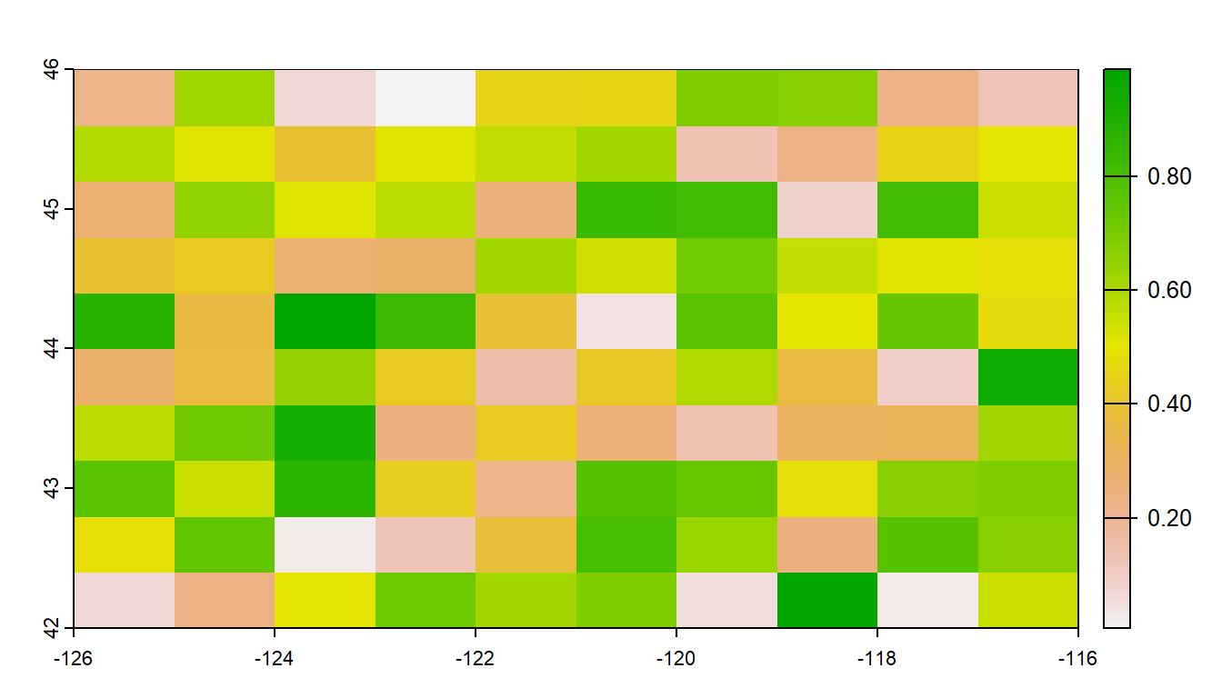

We can also overwrite the cell values for our raster:

values(myrast) <- 1:ncell(myrast)
values(myrast)[1:15]
#>  [1]  1  2  3  4  5  6  7  8  9 10 11 12 13 14 15

You can access raster values via direct indexing or line, column indexing - take a minute to see how this works using raster r we just created - the syntax is:

myrast[i]
myrast[line, column]

Exercise

How is terra data storage unlike a matrix in R? Try creating a matrix with same dimensions and values and compare with the terra raster you’ve created:

Solution

m <- matrix (1:100, nrow=10, ncol=10)
m[1,10]
#> [1] 91
myrast[1,10]
#>   lyr.1
#> 1    10
myrast[10]
#>   lyr.1
#> 1    10

1.4.2.2 Reading existing rasters on disk

raster_filepath = system.file("raster/srtm.tif", package = "spDataLarge")
my_rast = rast(raster_filepath)
nlyr(my_rast)
#> [1] 1
plot(my_rast)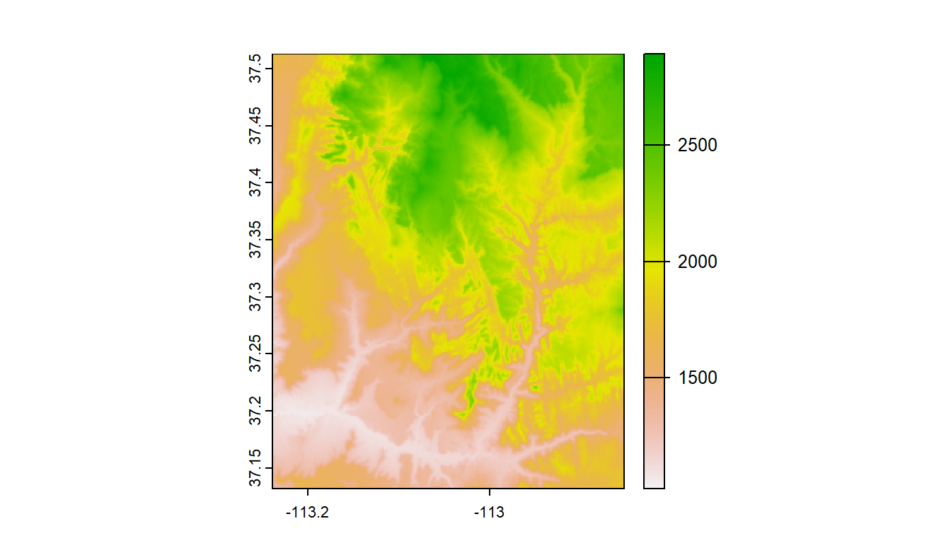

1.4.3 Multiband rasters

The spatRaster object in terra can hold multiple layers (similar to RasterBrick and RasterStack which were two additional classes in the raster package). These layers correspond to multispectral satellite imagery or a time-series raster.

landsat = system.file("raster/landsat.tif", package = "spDataLarge")
landsat = rast(landsat)
landsat
#> class       : SpatRaster 
#> dimensions  : 1428, 1128, 4  (nrow, ncol, nlyr)
#> resolution  : 30, 30  (x, y)
#> extent      : 301905, 335745, 4111245, 4154085  (xmin, xmax, ymin, ymax)
#> coord. ref. : WGS 84 / UTM zone 12N (EPSG:32612) 
#> source      : landsat.tif 
#> names       : landsat_1, landsat_2, landsat_3, landsat_4 
#> min values  :      7550,      6404,      5678,      5252 
#> max values  :     19071,     22051,     25780,     31961
plot(landsat)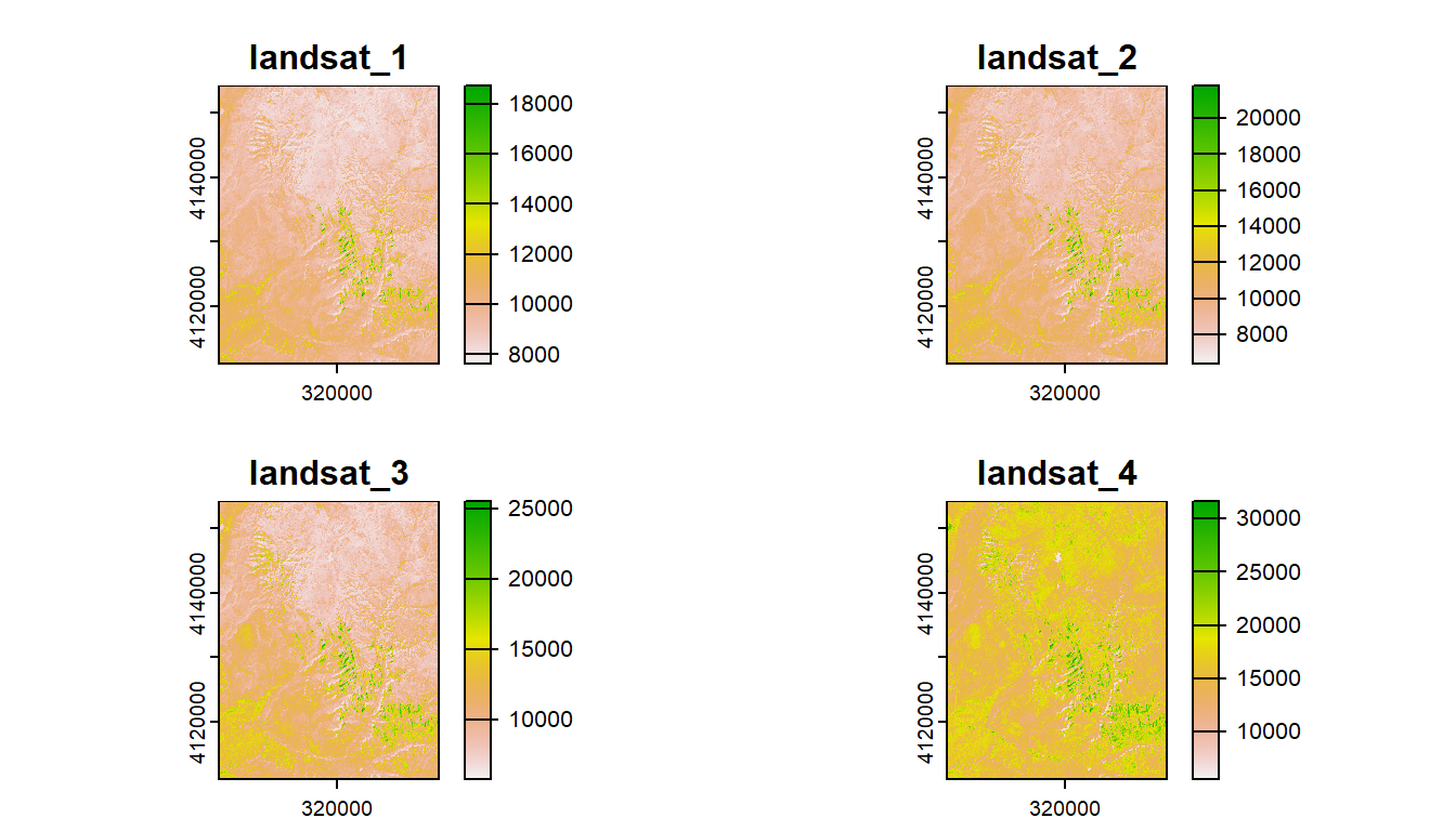

1.4.3.1 Raster data with `stars`

stars works with and stands for spatio-temporal arrays and can deal with more complex data types than either raster or terra such as rotated grids.

stars integrates with sf and many sf functions have methods for stars objects (i.e. st_bbox and st_transform) - this makes sense since they are both written by Edzer Pebesma. terra unfortunately has poor / no integration with sf - this is a big issue for me personally and I will likely look to stars long-term for my raster processing.

Basic example shown in stars vignette - reading in the 30m bands of a Landsat-7 image that comes with the stars package:

tif = system.file("tif/L7_ETMs.tif", package = "stars")
ls7 = read_stars(tif)
plot(ls7, axes = TRUE)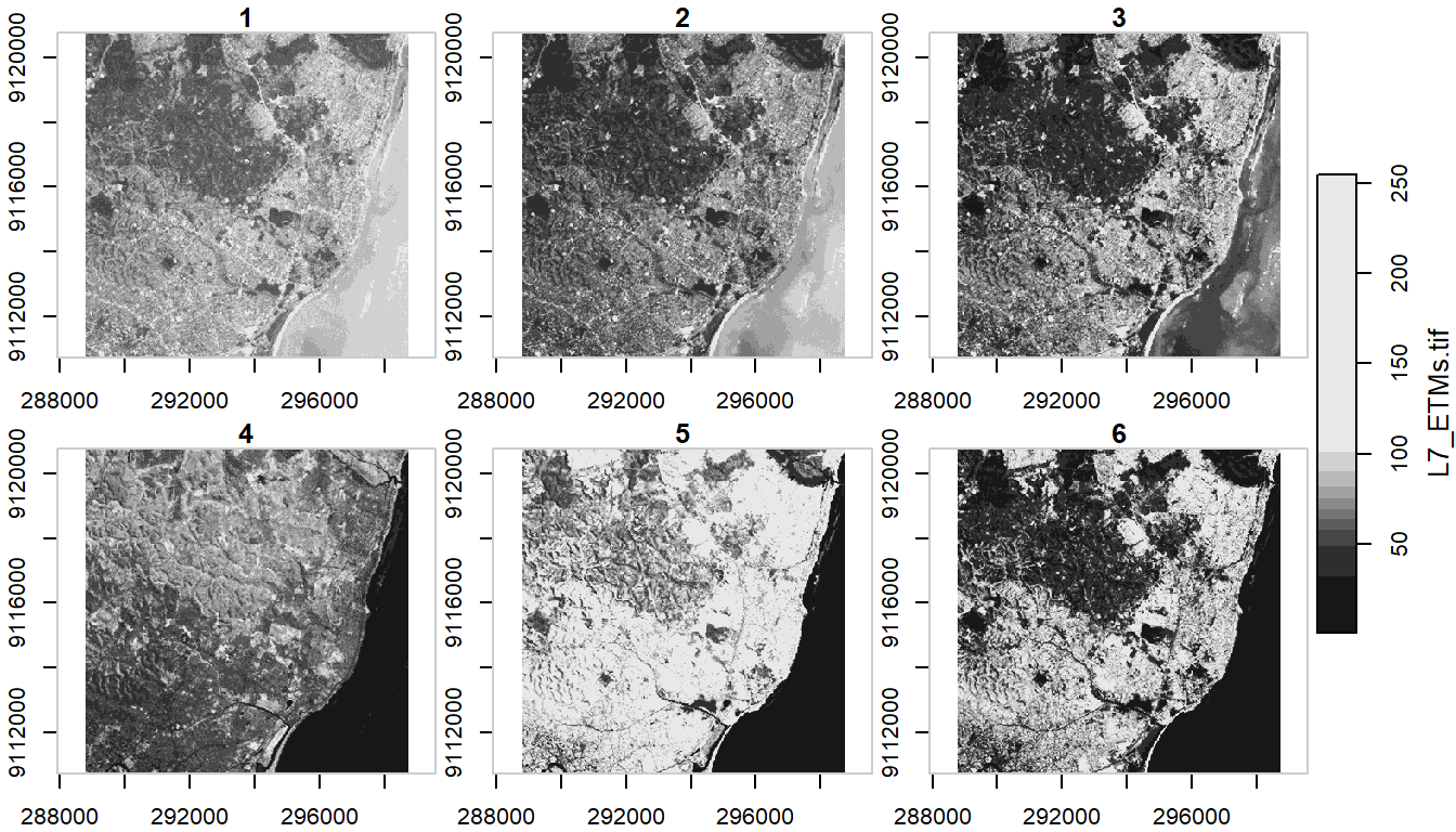

ls7 (landsat7) is an object with 3 dimensions (x,y and band) and 1 attribute

ls7
#> stars object with 3 dimensions and 1 attribute
#> attribute(s):
#>              Min. 1st Qu. Median     Mean 3rd Qu. Max.
#> L7_ETMs.tif     1      54     69 68.91242      86  255
#> dimension(s):
#>      from  to  offset delta                     refsys point x/y
#> x       1 349  288776  28.5 SIRGAS 2000 / UTM zone 25S FALSE [x]
#> y       1 352 9120761 -28.5 SIRGAS 2000 / UTM zone 25S FALSE [y]
#> band    1   6      NA    NA                         NA    NA

Note when we plotted above that the plot method with stars uses histogram stretching across all bands - we can also do stretching for each band individually:

plot(ls7, axes = TRUE, join_zlim = FALSE)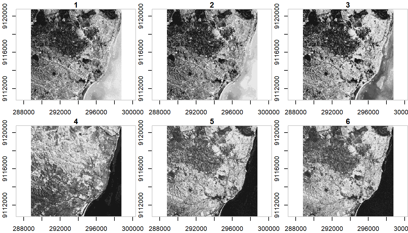

stars uses tidyverse methods for spatio-temporal arrays - an example of this is pulling out one band of an image using slice

ls7  |>  dplyr::slice(band, 6) -> band6
band6
#> stars object with 2 dimensions and 1 attribute
#> attribute(s):
#>              Min. 1st Qu. Median     Mean 3rd Qu. Max.
#> L7_ETMs.tif     1      32     60 59.97521      88  255
#> dimension(s):
#>   from  to  offset delta                     refsys point x/y
#> x    1 349  288776  28.5 SIRGAS 2000 / UTM zone 25S FALSE [x]
#> y    1 352 9120761 -28.5 SIRGAS 2000 / UTM zone 25S FALSE [y]

This gives us a lower-dimensional array of just band 6 from the Landsat7 image.

1.5 Coordinate Reference Systems

A CRS is made up of several components:

Coordinate system: The x,y grid that defines where your data lies in space
Horizontal and vertical units: The units describing grid along the x,y and possibly z axes
Datum: The modeled version of the shape of the earth
Projection details: If projected, the mathematical equation used to flatten objects from round surface (earth) to flat surface (paper or screen)

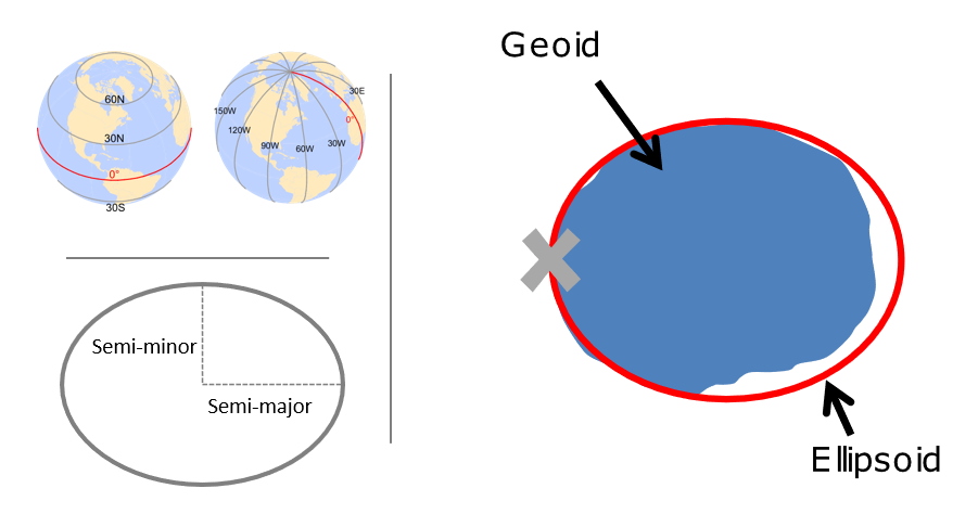
Source: https://mgimond.github.io/Spatial/chp09_0.html

1.5.1 The ellipsoid and geoid

The earth is a sphere, but more precisely, an ellipsoid, which is defined by two radii: - semi-major axis (equatorial radius) - semi-minor axis (polar radius)

The terms speroid and ellipsoid are used interchangeably. One particular spheroid is distinguished from another by the lengths of the semimajor and semiminor axes. Both GRS80 and WGS84 spheroids use semimajor and semiminor axes of 6,378,137 meters and 6,356,752 meters respectively (the semiminor axis differs by thousandths of meters between the two). You’ll encounter older spheroid / ellipsoids out there such as Clark 1866.

More precisely than an ellipsoid, though, we know that earth is a geoid - it is not perfectly smooth - and modelling the the undulations due to changes in gravitational pull for different locations is crucial to accuracy in a GIS. This is where a datum comes in - a datum is built on top of the selected spheroid and can incorporate local variations in elevation. We have many datums to choose from based on location of interest - in the US we would typically choose NAD83

1.5.2 Why you need to know about CRS working with spatial data in R:

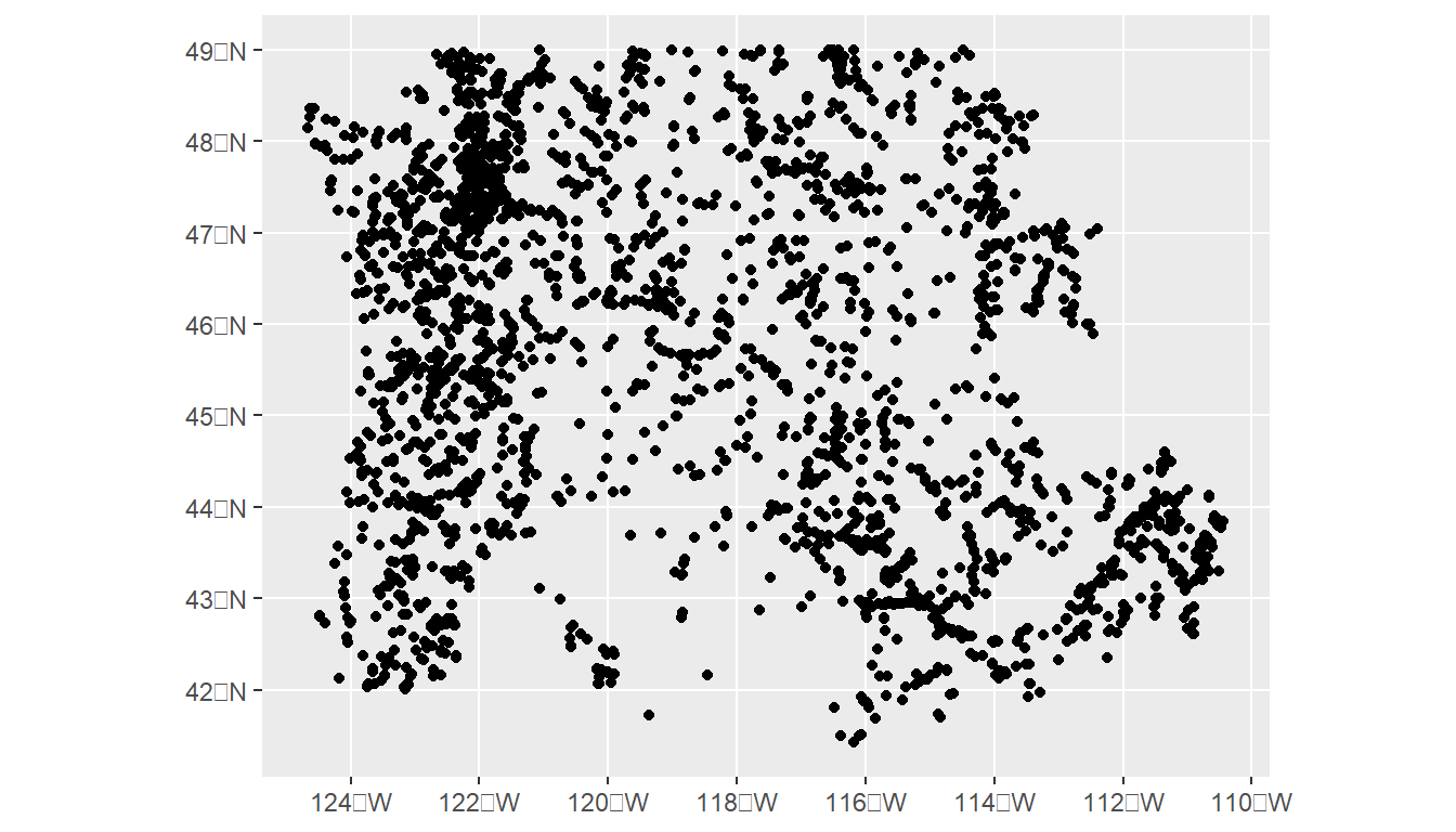
data(pnw)

gages = read_csv(system.file("extdata/Gages_flowdata.csv", package = "Rspatialworkshop"),show_col_types = FALSE)

gages_sf <- gages  |> 
  st_as_sf(coords = c("LON_SITE", "LAT_SITE"), crs = 4269, remove = FALSE)  |> 
  dplyr::select(STATION_NM,LON_SITE, LAT_SITE)

# Awesome, let's plot our gage data and state boundaries!
plot(pnw$geometry, axes=TRUE)
plot(gages_sf$geometry, col='red', add=TRUE)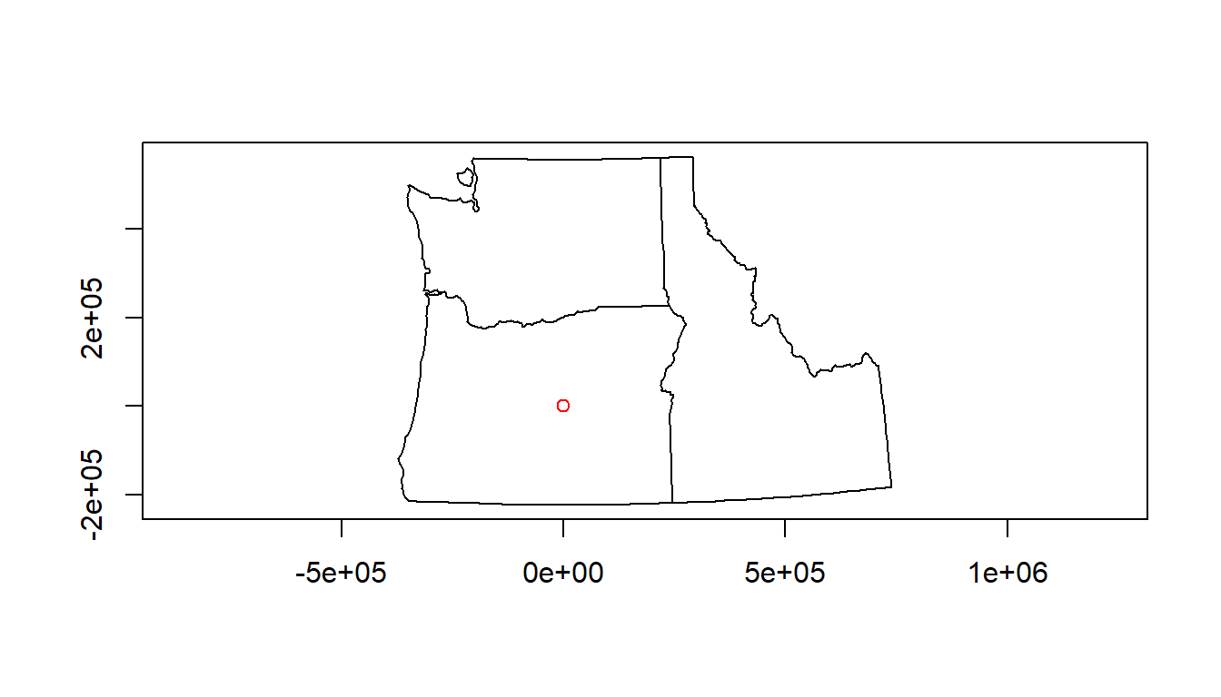

# um, what?

There is no ‘on-the-fly’ projection in R - you need to make sure you specify the CRS of your objects, and CRS needs to match for any spatial operations or you’ll get an error

spatialreference.org is your friend in R - chances are you will use it frequently working with spatial data in R.
projection Wizard is also really useful, as is epsg.io

1.5.3 Defining your coordinate reference system

A coordinate reference system for spatial data can be defined in different ways - for instance for the standard WGS84 coordinate system you could use:

Proj4
- +proj=longlat +ellps=WGS84 +datum=WGS84 +no_defs
OGC WKT
- GEOGCS["WGS 84",DATUM["WGS_1984",SPHEROID["WGS 84",6378137,298.257223563,AUTHORITY["EPSG","7030"]],AUTHORITY["EPSG","6326"]],PRIMEM["Greenwich",0,AUTHORITY["EPSG","8901"]],UNIT["degree",0.01745329251994328,AUTHORITY["EPSG","9122"]],AUTHORITY["EPSG","4326"]]
ESRI WKT
- GEOGCS["GCS_WGS_1984",DATUM["D_WGS_1984",SPHEROID["WGS_1984",6378137,298.257223563]],PRIMEM["Greenwich",0],UNIT["Degree",0.017453292519943295]]
‘authority:code’ identifier
- EPSG:4326

Proj4 used to be the standard crs identifier in R but the preferable way is to use the AUTHORITY:CODE method which sf as well as software like QGIS will recognize. The AUTHORITY:CODE method is durable and easily discoverable online.

The WKT representation of EPSG:4326 in sf is:

sf::st_crs('EPSG:4326')
#> Coordinate Reference System:
#>   User input: EPSG:4326 
#>   wkt:
#> GEOGCRS["WGS 84",
#>     ENSEMBLE["World Geodetic System 1984 ensemble",
#>         MEMBER["World Geodetic System 1984 (Transit)"],
#>         MEMBER["World Geodetic System 1984 (G730)"],
#>         MEMBER["World Geodetic System 1984 (G873)"],
#>         MEMBER["World Geodetic System 1984 (G1150)"],
#>         MEMBER["World Geodetic System 1984 (G1674)"],
#>         MEMBER["World Geodetic System 1984 (G1762)"],
#>         MEMBER["World Geodetic System 1984 (G2139)"],
#>         ELLIPSOID["WGS 84",6378137,298.257223563,
#>             LENGTHUNIT["metre",1]],
#>         ENSEMBLEACCURACY[2.0]],
#>     PRIMEM["Greenwich",0,
#>         ANGLEUNIT["degree",0.0174532925199433]],
#>     CS[ellipsoidal,2],
#>         AXIS["geodetic latitude (Lat)",north,
#>             ORDER[1],
#>             ANGLEUNIT["degree",0.0174532925199433]],
#>         AXIS["geodetic longitude (Lon)",east,
#>             ORDER[2],
#>             ANGLEUNIT["degree",0.0174532925199433]],
#>     USAGE[
#>         SCOPE["Horizontal component of 3D system."],
#>         AREA["World."],
#>         BBOX[-90,-180,90,180]],
#>     ID["EPSG",4326]]

1.5.4 Projected coordinate systems

Typically we want to work with data that is projected. Projected coordinate systems (which are based on Cartesian coordinates) have: an origin, an x axis, a y axis, and a linear unit of measure. Going from geographic coordinates to a projected coordinate reference systems requires mathematical transformations.

Four spatial properties of projected coordinate systems that are subject to distortion are: shape, area, distance and direction. A map that preserves shape is called conformal; one that preserves area is called equal-area; one that preserves distance is called equidistant; and one that preserves direction is called azimuthal (from https://mgimond.github.io/Spatial/chp09_0.html.

The takeaway from all this is you need to be aware of the crs for your objects in R, make sure they are projected if appropriate and in a projection that optimizes properties you are interested in, and objects you are analyzing or mapping together need to be in same crs.

Going back to our original example, we can transform crs of objects to work with them together:

# Check our coordinate reference systems
st_crs(gages_sf)
#> Coordinate Reference System:
#>   User input: EPSG:4269 
#>   wkt:
#> GEOGCRS["NAD83",
#>     DATUM["North American Datum 1983",
#>         ELLIPSOID["GRS 1980",6378137,298.257222101,
#>             LENGTHUNIT["metre",1]]],
#>     PRIMEM["Greenwich",0,
#>         ANGLEUNIT["degree",0.0174532925199433]],
#>     CS[ellipsoidal,2],
#>         AXIS["geodetic latitude (Lat)",north,
#>             ORDER[1],
#>             ANGLEUNIT["degree",0.0174532925199433]],
#>         AXIS["geodetic longitude (Lon)",east,
#>             ORDER[2],
#>             ANGLEUNIT["degree",0.0174532925199433]],
#>     USAGE[
#>         SCOPE["Geodesy."],
#>         AREA["North America - onshore and offshore: Canada - Alberta; British Columbia; Manitoba; New Brunswick; Newfoundland and Labrador; Northwest Territories; Nova Scotia; Nunavut; Ontario; Prince Edward Island; Quebec; Saskatchewan; Yukon. Puerto Rico. United States (USA) - Alabama; Alaska; Arizona; Arkansas; California; Colorado; Connecticut; Delaware; Florida; Georgia; Hawaii; Idaho; Illinois; Indiana; Iowa; Kansas; Kentucky; Louisiana; Maine; Maryland; Massachusetts; Michigan; Minnesota; Mississippi; Missouri; Montana; Nebraska; Nevada; New Hampshire; New Jersey; New Mexico; New York; North Carolina; North Dakota; Ohio; Oklahoma; Oregon; Pennsylvania; Rhode Island; South Carolina; South Dakota; Tennessee; Texas; Utah; Vermont; Virginia; Washington; West Virginia; Wisconsin; Wyoming. US Virgin Islands. British Virgin Islands."],
#>         BBOX[14.92,167.65,86.46,-47.74]],
#>     ID["EPSG",4269]]
st_crs(pnw)
#> Coordinate Reference System:
#>   User input: +proj=aea +lat_1=41 +lat_2=47 +lat_0=44 +lon_0=-120 +x_0=0 +y_0=0 +ellps=GRS80 +datum=NAD83 +units=m +no_defs 
#>   wkt:
#> PROJCRS["unknown",
#>     BASEGEOGCRS["unknown",
#>         DATUM["North American Datum 1983",
#>             ELLIPSOID["GRS 1980",6378137,298.257222101,
#>                 LENGTHUNIT["metre",1]],
#>             ID["EPSG",6269]],
#>         PRIMEM["Greenwich",0,
#>             ANGLEUNIT["degree",0.0174532925199433],
#>             ID["EPSG",8901]]],
#>     CONVERSION["unknown",
#>         METHOD["Albers Equal Area",
#>             ID["EPSG",9822]],
#>         PARAMETER["Latitude of false origin",44,
#>             ANGLEUNIT["degree",0.0174532925199433],
#>             ID["EPSG",8821]],
#>         PARAMETER["Longitude of false origin",-120,
#>             ANGLEUNIT["degree",0.0174532925199433],
#>             ID["EPSG",8822]],
#>         PARAMETER["Latitude of 1st standard parallel",41,
#>             ANGLEUNIT["degree",0.0174532925199433],
#>             ID["EPSG",8823]],
#>         PARAMETER["Latitude of 2nd standard parallel",47,
#>             ANGLEUNIT["degree",0.0174532925199433],
#>             ID["EPSG",8824]],
#>         PARAMETER["Easting at false origin",0,
#>             LENGTHUNIT["metre",1],
#>             ID["EPSG",8826]],
#>         PARAMETER["Northing at false origin",0,
#>             LENGTHUNIT["metre",1],
#>             ID["EPSG",8827]]],
#>     CS[Cartesian,2],
#>         AXIS["(E)",east,
#>             ORDER[1],
#>             LENGTHUNIT["metre",1,
#>                 ID["EPSG",9001]]],
#>         AXIS["(N)",north,
#>             ORDER[2],
#>             LENGTHUNIT["metre",1,
#>                 ID["EPSG",9001]]]]
# Are they equal?
st_crs(gages_sf)==st_crs(pnw)
#> [1] FALSE
# transform one to the other
gages_sf <- st_transform(gages_sf, st_crs(pnw))
ggplot() + 
  geom_sf(data = gages_sf,  color="blue") +
  geom_sf(data = pnw,  color="black", fill=NA) +
  labs(title="USGS Stream Gages in the Pacific Northwest") +
  theme_bw()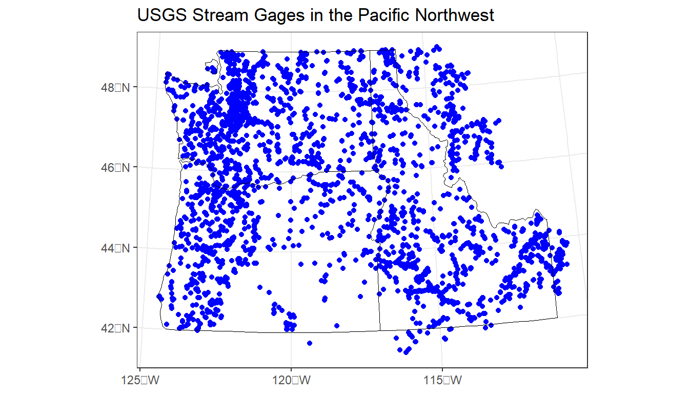

Exercise

Re-project both the PNW state polygons and the stream gages to a different projected CRS - I suggest UTM zone 11, or perhaps Oregon Lambert, but choose your own. Use resources I list above to find a projection and get it’s specification to use in R to re-project both sf objects, then plot together either in base R or ggplot.

Solution

My solution:

# first I save the previous plot so we can view it alongside our update:
p1 <-ggplot() + 
  geom_sf(data=gages_sf,  color="blue") +
  geom_sf(data=pnw,  color="black", fill=NA) +
  labs(title="Albers Equal Area") +
  theme_bw()
# You can fully specify the WKT:
utmz11 <- 'PROJCS["NAD83(CSRS98) / UTM zone 11N (deprecated)",GEOGCS["NAD83(CSRS98)",DATUM["NAD83_Canadian_Spatial_Reference_System",SPHEROID["GRS 1980",6378137,298.257222101,AUTHORITY["EPSG","7019"]],TOWGS84[0,0,0,0,0,0,0],AUTHORITY["EPSG","6140"]],PRIMEM["Greenwich",0,AUTHORITY["EPSG","8901"]],UNIT["degree",0.0174532925199433,AUTHORITY["EPSG","9108"]],AUTHORITY["EPSG","4140"]],UNIT["metre",1,AUTHORITY["EPSG","9001"]],PROJECTION["Transverse_Mercator"],PARAMETER["latitude_of_origin",0],PARAMETER["central_meridian",-117],PARAMETER["scale_factor",0.9996],PARAMETER["false_easting",500000],PARAMETER["false_northing",0],AUTHORITY["EPSG","2153"],AXIS["Easting",EAST],AXIS["Northing",NORTH]]'

# or you can simply provide the EPSG code:
utmz11 <- 2153
gages_sf <- st_transform(gages_sf, utmz11)
pnw <- st_transform(pnw, utmz11)
p2 <- ggplot() + 
  geom_sf(data=gages_sf,  color="blue") +
  geom_sf(data=pnw,  color="black", fill=NA) +
  labs(title="UTM Zone 11") +
  theme_bw() 
plot_grid(p1, p2)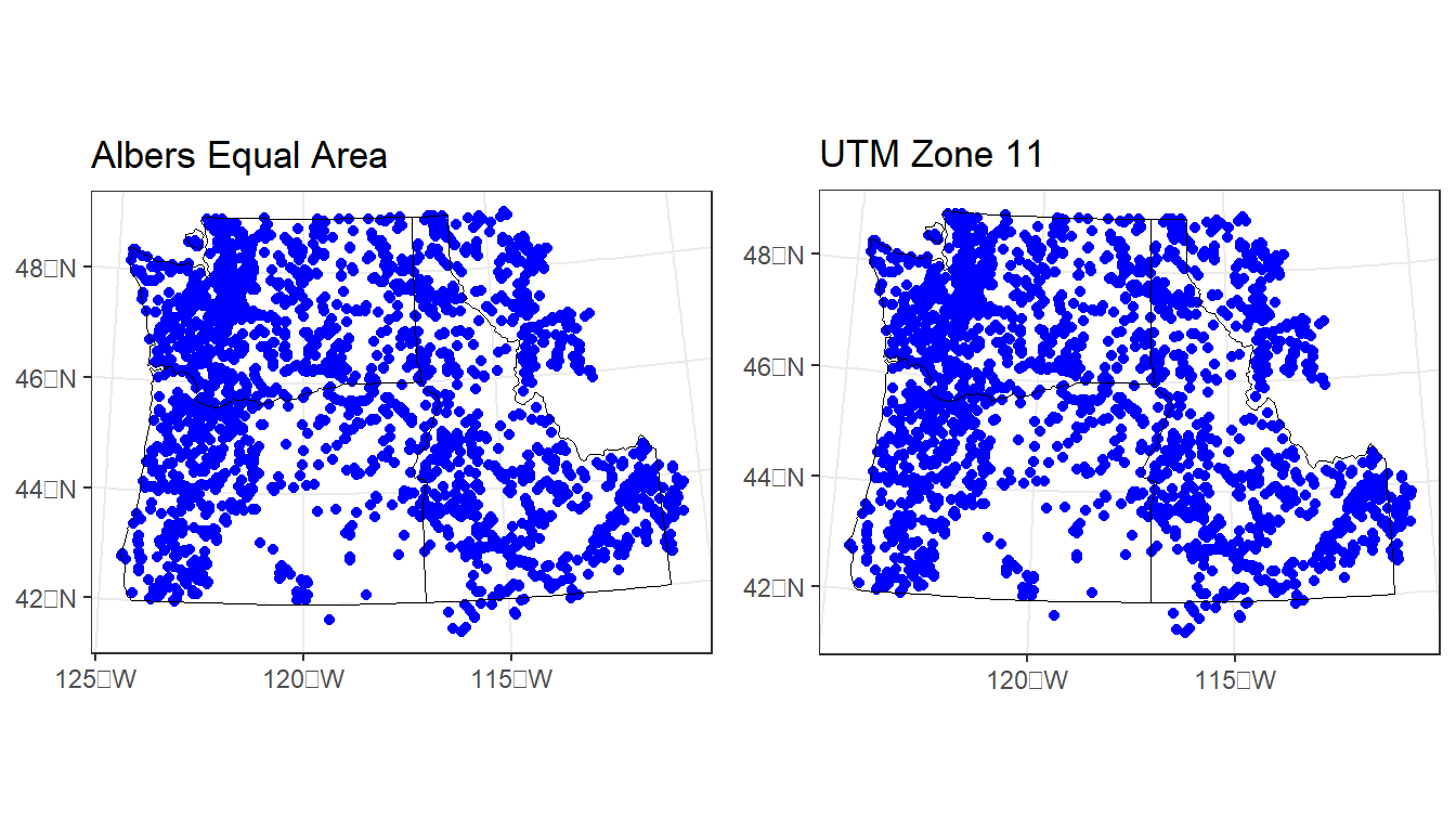

1.5.5 Projecting

For spatial operations in R, raster or vector, we always need to make sure objects are in an appropriate crs and in the same crs as one another.

We’ll use the elevation data and a polygon feature for Crater Lake from the Rspatialworkshop package for this example.

data(CraterLake)
raster_filepath <- system.file("extdata", "elevation.tif", package = "Rspatialworkshop")
elevation <- terra::rast(raster_filepath)

:::{.callout-note} #### Exercise 1. Find the projection of both the Crater Lake spatial polygon feature and the elevation raster 2. Are they the same? Should we project one to the other, or apply a new projection?

:::{.callout-note collapse=“true”} #### Solution 1. Check the CRS of each feature and test for equality

crs(elevation)
#> [1] "GEOGCRS[\"WGS 84\",\n    ENSEMBLE[\"World Geodetic System 1984 ensemble\",\n        MEMBER[\"World Geodetic System 1984 (Transit)\"],\n        MEMBER[\"World Geodetic System 1984 (G730)\"],\n        MEMBER[\"World Geodetic System 1984 (G873)\"],\n        MEMBER[\"World Geodetic System 1984 (G1150)\"],\n        MEMBER[\"World Geodetic System 1984 (G1674)\"],\n        MEMBER[\"World Geodetic System 1984 (G1762)\"],\n        MEMBER[\"World Geodetic System 1984 (G2139)\"],\n        ELLIPSOID[\"WGS 84\",6378137,298.257223563,\n            LENGTHUNIT[\"metre\",1]],\n        ENSEMBLEACCURACY[2.0]],\n    PRIMEM[\"Greenwich\",0,\n        ANGLEUNIT[\"degree\",0.0174532925199433]],\n    CS[ellipsoidal,2],\n        AXIS[\"geodetic latitude (Lat)\",north,\n            ORDER[1],\n            ANGLEUNIT[\"degree\",0.0174532925199433]],\n        AXIS[\"geodetic longitude (Lon)\",east,\n            ORDER[2],\n            ANGLEUNIT[\"degree\",0.0174532925199433]],\n    USAGE[\n        SCOPE[\"Horizontal component of 3D system.\"],\n        AREA[\"World.\"],\n        BBOX[-90,-180,90,180]],\n    ID[\"EPSG\",4326]]"
st_crs(CraterLake)
#> Coordinate Reference System:
#>   User input: WGS 84 
#>   wkt:
#> GEOGCRS["WGS 84",
#>     DATUM["World Geodetic System 1984",
#>         ELLIPSOID["WGS 84",6378137,298.257223563,
#>             LENGTHUNIT["metre",1]]],
#>     PRIMEM["Greenwich",0,
#>         ANGLEUNIT["degree",0.0174532925199433]],
#>     CS[ellipsoidal,2],
#>         AXIS["geodetic latitude (Lat)",north,
#>             ORDER[1],
#>             ANGLEUNIT["degree",0.0174532925199433]],
#>         AXIS["geodetic longitude (Lon)",east,
#>             ORDER[2],
#>             ANGLEUNIT["degree",0.0174532925199433]],
#>     ID["EPSG",4326]]
st_crs(CraterLake) == crs(elevation)
#> [1] FALSE
st_crs(CraterLake)$wkt == crs(elevation)
#> [1] FALSE

They share the same EPSG code, but are parameterized slightly differently for each - the crs function in terra does not include the input list item that st_crs in sf does - they are the same though as demonstrated when specifying the wkt item only from st_crs(CraterLake)
Each feature is in WGS84, an unprojected CRS - for most operations, we would prefer to have them in a projected CRS

Exercise

Find an appropriate area-preserving projection using Projection Wizard or spatialreference.org or any means you prefer and project both Crater Lake and elevation to this CRS.

Solution

Here I’ll apply a custom Transverse Mercator I found the WKT representation for using Projection Wizard. Another good projection would be UTM zone 10N or UTM zone 11N

tranvmerc <- 'PROJCS["ProjWiz_Custom_Transverse_Mercator", GEOGCS["GCS_WGS_1984", DATUM["D_WGS_1984", SPHEROID["WGS_1984",6378137.0,298.257223563]], PRIMEM["Greenwich",0.0], UNIT["Degree",0.0174532925199433]],PROJECTION["Transverse_Mercator"],PARAMETER["False_Easting",500000],PARAMETER["False_Northing",0.0],PARAMETER["Central_Meridian",-483.2226562],PARAMETER["Scale_Factor",0.9996],PARAMETER["Latitude_Of_Origin",0.0],UNIT["Meter",1.0]]'
elevation_tm <- project(elevation, tranvmerc, method = "bilinear")
crs(elevation_tm)
#> [1] "PROJCRS[\"ProjWiz_Custom_Transverse_Mercator\",\n    BASEGEOGCRS[\"WGS 84\",\n        DATUM[\"World Geodetic System 1984\",\n            ELLIPSOID[\"WGS 84\",6378137,298.257223563,\n                LENGTHUNIT[\"metre\",1]],\n            ID[\"EPSG\",6326]],\n        PRIMEM[\"Greenwich\",0,\n            ANGLEUNIT[\"Degree\",0.0174532925199433]]],\n    CONVERSION[\"unnamed\",\n        METHOD[\"Transverse Mercator\",\n            ID[\"EPSG\",9807]],\n        PARAMETER[\"Latitude of natural origin\",0,\n            ANGLEUNIT[\"Degree\",0.0174532925199433],\n            ID[\"EPSG\",8801]],\n        PARAMETER[\"Longitude of natural origin\",-483.2226562,\n            ANGLEUNIT[\"Degree\",0.0174532925199433],\n            ID[\"EPSG\",8802]],\n        PARAMETER[\"Scale factor at natural origin\",0.9996,\n            SCALEUNIT[\"unity\",1],\n            ID[\"EPSG\",8805]],\n        PARAMETER[\"False easting\",500000,\n            LENGTHUNIT[\"metre\",1],\n            ID[\"EPSG\",8806]],\n        PARAMETER[\"False northing\",0,\n            LENGTHUNIT[\"metre\",1],\n            ID[\"EPSG\",8807]]],\n    CS[Cartesian,2],\n        AXIS[\"(E)\",east,\n            ORDER[1],\n            LENGTHUNIT[\"metre\",1,\n                ID[\"EPSG\",9001]]],\n        AXIS[\"(N)\",north,\n            ORDER[2],\n            LENGTHUNIT[\"metre\",1,\n                ID[\"EPSG\",9001]]]]"
CraterLake_tm <- st_transform(CraterLake,tranvmerc)

1.5.6 `S2` class

It’s important to note a recent change in R spatial with spherical geometry. Since sf version 1.0.0, R supports spherical geometry operations by default via its interface to Google’s S2 spherical geometry engine and the s2 interface package. S2 is perhaps best known as an example of a Discrete Global Grid System (DGGS). Another example of this is the H3 global hexagonal hierarchical spatial index.

sf can run with s2 on or off and by default the S2 geometry engine is turned on:

sf::sf_use_s2()
#> [1] TRUE

See the Geocomputation with R s2 section for further details

Note

There are sometimes good reasons for turning S2 off during an R session. See issue 1771 in sf’s GitHub repo - the default behavior can make code that would work with S2 turned off (and with older versions of sf) fail.

Situations that can cause problems include operations on polygons that are not valid according to S2’s stricter definition. If you see error message such as #> Error in s2_geography_from_wkb ... you may want to turn s2 off and try your operation again, perhaps turning of s2 and running a topology clean operation like st_make_valid().

1.6 Geographic Data Input/Output (I/O)

There are several ways we typically get spatial data into R:
- Load spatial files we have on our machine or from remote source
- Load spatial data that is part of an R package
- Grab data using API (often making use of particular R packages)
- Converting flat files with x,y data to spatial data
- Geocoding data (we saw example of this at beginning)

For reading and writing vector and raster data in R, the several main packages we’ll look at are:

sffor vector formats such as ESRI Shapefiles, GeoJSON, and GPX - sf uses OGR, which is a library under the GDAL source tree,under the hood
terra or stars for raster formats such as GeoTIFF or ESRI or ASCII grid using GDAL under the hood

We can quickly discover supported I/O vector formats either via sf or rgdal:

print(paste0('There are ',st_drivers("vector")  |>  nrow(), ' vector drivers available using st_read or read_sf'))
#> [1] "There are 67 vector drivers available using st_read or read_sf"
kable(head(st_drivers(what='vector'),n=5))

	name	long_name	write	copy	is_raster	is_vector	vsi
ESRIC	ESRIC	Esri Compact Cache	FALSE	FALSE	TRUE	TRUE	TRUE
netCDF	netCDF	Network Common Data Format	TRUE	TRUE	TRUE	TRUE	FALSE
PDS4	PDS4	NASA Planetary Data System 4	TRUE	TRUE	TRUE	TRUE	TRUE
VICAR	VICAR	MIPL VICAR file	TRUE	TRUE	TRUE	TRUE	TRUE
JP2OpenJPEG	JP2OpenJPEG	JPEG-2000 driver based on OpenJPEG library	FALSE	TRUE	TRUE	TRUE	TRUE

As well as I/O raster formats via sf:

print(paste0('There are ',st_drivers(what='raster')  |>  nrow(), ' raster drivers available'))
#> [1] "There are 141 raster drivers available"
kable(head(st_drivers(what='raster'),n=5))

	name	long_name	write	copy	is_raster	is_vector	vsi
VRT	VRT	Virtual Raster	TRUE	TRUE	TRUE	FALSE	TRUE
DERIVED	DERIVED	Derived datasets using VRT pixel functions	FALSE	FALSE	TRUE	FALSE	FALSE
GTiff	GTiff	GeoTIFF	TRUE	TRUE	TRUE	FALSE	TRUE
COG	COG	Cloud optimized GeoTIFF generator	FALSE	TRUE	TRUE	FALSE	TRUE
NITF	NITF	National Imagery Transmission Format	TRUE	TRUE	TRUE	FALSE	TRUE

1.6.1 Reading in vector data

sf can be used to read numerous file types:

Shapefiles
Geodatabases
Geopackages
Geojson
Spatial database files

1.6.1.1 Shapefiles

Typically working with vector GIS data we work with ESRI shapefiles or geodatabases - here we have an example of how one would read in a shapefile using sf:

citylims <- read_sf(system.file("extdata/city_limits.shp", package = "Rspatialworkshop"))

options(scipen=3)
plot(citylims$geometry, axes=T, main='Oregon City Limits') # plot it!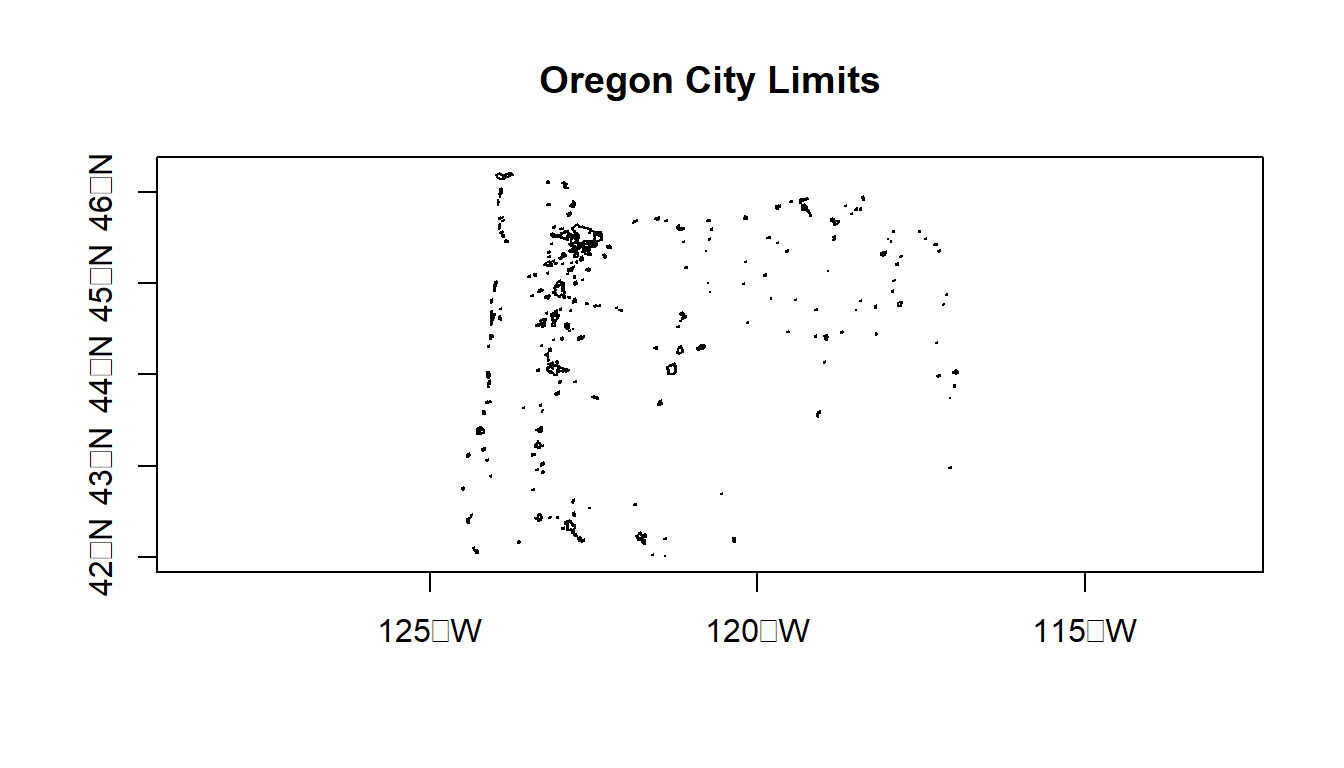

Exercise

st_read versus read_sf - throughout this section I’ve used read_sf and st_read - I typically use read_sf - why would that be a good practice?

Solution

read_sf is an sf alternative to st_read (see this section 1.2.2). Try reading in citylims data above using read_sf and notice difference, and check out help(read_sf). read_sf and write_sf are simply aliases for st_read and st_write with modified default arguments. Big differences are:

stringsAsFactors = FALSE
quiet = TRUE
as_tibble = TRUE

Note that stringsAsFactors = FALSE is the new default in R versions >= 4.0

1.6.1.2 Geodatabases

We use st_read or read_sf similarly for reading in an ESRI file geodatabase feature:

# List all feature classes in a file geodatabase
st_layers(system.file("extdata/StateParkBoundaries.gdb", package = "Rspatialworkshop"))
#> Driver: OpenFileGDB 
#> Available layers:
#>            layer_name geometry_type features fields                 crs_name
#> 1 StateParkBoundaries Multi Polygon      431     15 WGS 84 / Pseudo-Mercator
fgdb = system.file("extdata/StateParkBoundaries.gdb", package = "Rspatialworkshop")
# Read the feature class
parks <- st_read(dsn=fgdb,layer="StateParkBoundaries")
#> Reading layer `StateParkBoundaries' from data source 
#>   `C:\Program Files\R\R-4.2.2\library\Rspatialworkshop\extdata\StateParkBoundaries.gdb' 
#>   using driver `OpenFileGDB'
#> Simple feature collection with 431 features and 15 fields
#> Geometry type: MULTIPOLYGON
#> Dimension:     XY
#> Bounding box:  xmin: -13866300 ymin: 5159950 xmax: -13019620 ymax: 5818601
#> Projected CRS: WGS 84 / Pseudo-Mercator
ggplot(parks) + geom_sf()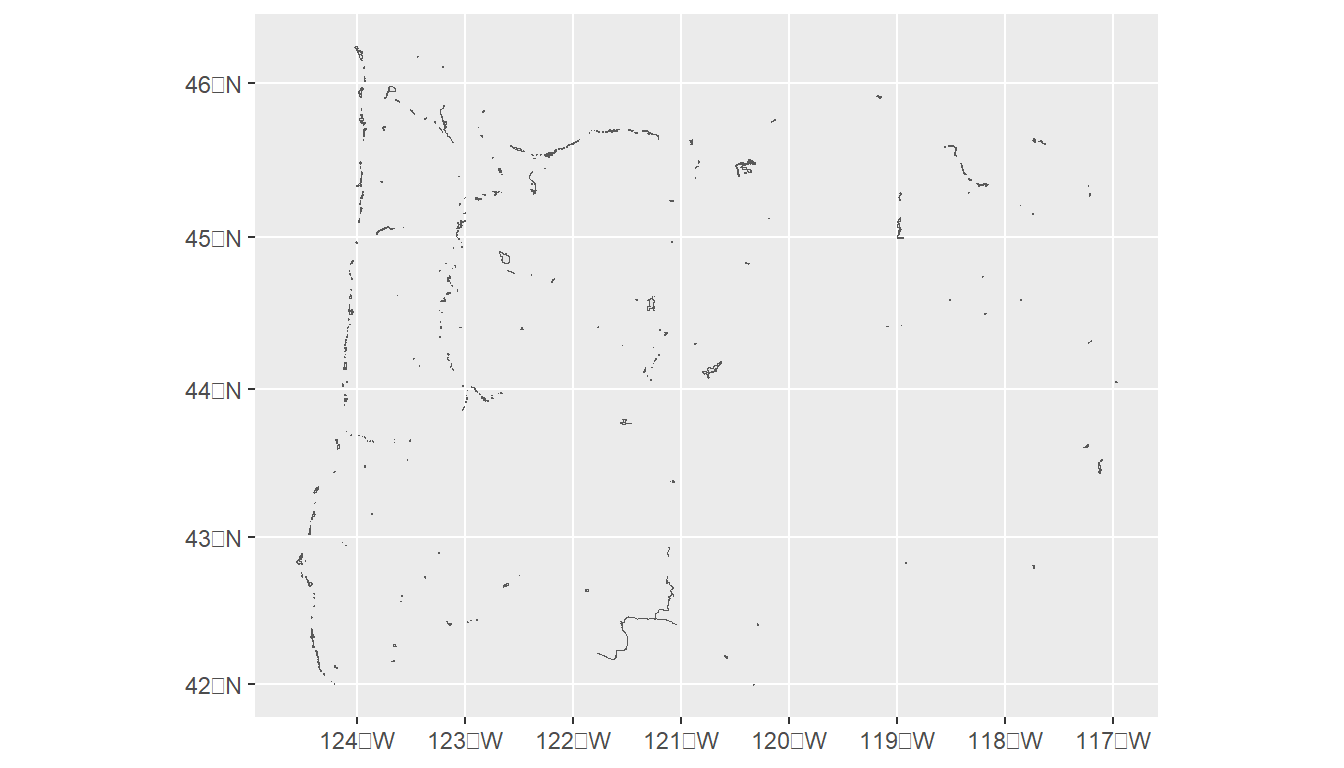

1.6.2 Geopackages

Another spatial file format is the geopackage. Let’s try a quick read and write of geopackage data. First we’ll read in a geopackage using data that comes with sf using dplyr syntax just to show something a bit different and use read_sf as an alternative to st_read. You may want to try writing the data back out as a geopackage as well.

nc <- system.file("gpkg/nc.gpkg", package="sf")  |>  read_sf() # reads in
glimpse(nc)
#> Rows: 100
#> Columns: 15
#> $ AREA      <dbl> 0.114, 0.061, 0.143, 0.070, 0.153, 0.097, 0.062, 0.091, 0…
#> $ PERIMETER <dbl> 1.442, 1.231, 1.630, 2.968, 2.206, 1.670, 1.547, 1.284, 1…
#> $ CNTY_     <dbl> 1825, 1827, 1828, 1831, 1832, 1833, 1834, 1835, 1836, 183…
#> $ CNTY_ID   <dbl> 1825, 1827, 1828, 1831, 1832, 1833, 1834, 1835, 1836, 183…
#> $ NAME      <chr> "Ashe", "Alleghany", "Surry", "Currituck", "Northampton",…
#> $ FIPS      <chr> "37009", "37005", "37171", "37053", "37131", "37091", "37…
#> $ FIPSNO    <dbl> 37009, 37005, 37171, 37053, 37131, 37091, 37029, 37073, 3…
#> $ CRESS_ID  <int> 5, 3, 86, 27, 66, 46, 15, 37, 93, 85, 17, 79, 39, 73, 91,…
#> $ BIR74     <dbl> 1091, 487, 3188, 508, 1421, 1452, 286, 420, 968, 1612, 10…
#> $ SID74     <dbl> 1, 0, 5, 1, 9, 7, 0, 0, 4, 1, 2, 16, 4, 4, 4, 18, 3, 4, 1…
#> $ NWBIR74   <dbl> 10, 10, 208, 123, 1066, 954, 115, 254, 748, 160, 550, 124…
#> $ BIR79     <dbl> 1364, 542, 3616, 830, 1606, 1838, 350, 594, 1190, 2038, 1…
#> $ SID79     <dbl> 0, 3, 6, 2, 3, 5, 2, 2, 2, 5, 2, 5, 4, 4, 6, 17, 4, 7, 1,…
#> $ NWBIR79   <dbl> 19, 12, 260, 145, 1197, 1237, 139, 371, 844, 176, 597, 13…
#> $ geom      <MULTIPOLYGON [°]> MULTIPOLYGON (((-81.47276 3..., MULTIPOLYGON…

Exercise

What are a couple advantages of geopackages over shapefiles?

Solution

Some thoughts here, main ones probably:

geopackages avoid mult-file format of shapefiles
geopackages avoid the 2gb limit of shapefiles
geopackages are open-source and follow OGC standards
lighter in file size than shapefiles
geopackages avoid the 10-character limit to column headers in shapefile attribute tables (stored in archaic .dbf files)

1.6.2.1 Open spatial data sources

There is a wealth of open spatial data accessible online now via static URLs or APIs - a few examples include Data.gov, NASA SECAC Portal, Natural Earth, UNEP GEOdata, and countless others listed here at Free GIS Data

1.6.2.2 Spatial data from R packages

There are also a number of R packages written specifically to provide access to geospatial data - below are a few and we’ll step through some examples of pulling in data using some of these packages.

Example R packages for spatial data retrieval.
Package name	Description
USABoundaries	Provide historic and contemporary boundaries of the US
tigris	Download and use US Census TIGER/Line Shapefiles in R
tidycensus	Uses Census American Community API to return tidyverse and optionally sf ready data frames
FedData	Functions for downloading geospatial data from several federal sources
elevatr	Access elevation data from various APIs (by Jeff Hollister)
getlandsat	Provides access to Landsat 8 data.
osmdata	Download and import of OpenStreetMap data.
raster	The `getData()` function downloads and imports administrative country, SRTM/ASTER elevation, WorldClim data.
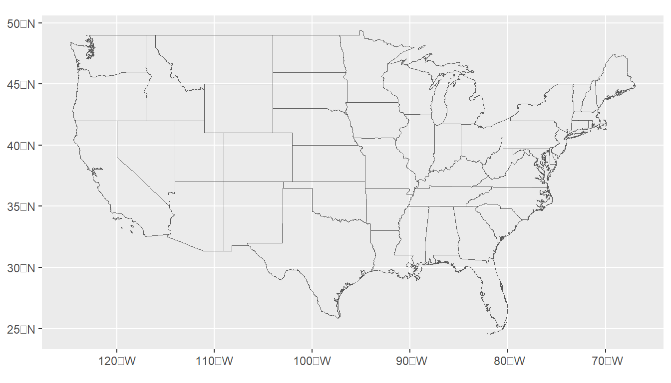
rnaturalearth	Functions to download Natural Earth vector and raster data, including world country borders.
rnoaa	An R interface to National Oceanic and Atmospheric Administration (NOAA) climate data.
rWBclimate	An access to the World Bank climate data.

Below is an example of pulling in US states using the rnaturalearth package - note that the default is to pull in data as sp objects and we coerce to sf. Also take a look at the chained operation using dplyr. Try changing the filter or a parameter in ggplot.

states <- ne_states(country = 'United States of America')
states_sf <- st_as_sf(states)
states_sf  |>  
  dplyr::filter(!name %in% c('Hawaii','Alaska') & !is.na(name)) |> 
  ggplot() + geom_sf(fill=NA)

1.6.2.3 Read in OpenStreetMap data

The osmdata package is a fantastic resource for leveraging the OpenStreetMap (OSM) database.

First we’ll find available tags to get foot paths to plot

head(available_tags("highway")) # get rid of head when you run - just used to truncate output
#> # A tibble: 6 × 2
#>   Key     Value       
#>   <chr>   <chr>       
#> 1 highway bridleway   
#> 2 highway bus_guideway
#> 3 highway bus_stop    
#> 4 highway busway      
#> 5 highway construction
#> 6 highway corridor

footway <- opq(bbox = "corvallis oregon") %>% 
  add_osm_feature(key = "highway", value = c("footway","cycleway","path", "path","pedestrian","track")) %>% 
  osmdata_sf()
footway <- footway$osm_lines

rstrnts <- opq(bbox = "corvallis oregon") %>% 
    add_osm_feature(key = "amenity", value = "restaurant") %>%
    osmdata_sf()
rstrnts <- rstrnts$osm_points

mapview(footway$geometry) + mapview(rstrnts)

Exercise

Take a minute and try pulling in data of your own for your own area and plotting using osmdata

1.6.3 Reading in Raster data

1.6.4 `terra` package

Load stock elevation .tif file that comes with package

f <- system.file("ex/elev.tif", package="terra")
elev <- rast(f)
barplot(elev, digits=-1, las=2, ylab="Frequency")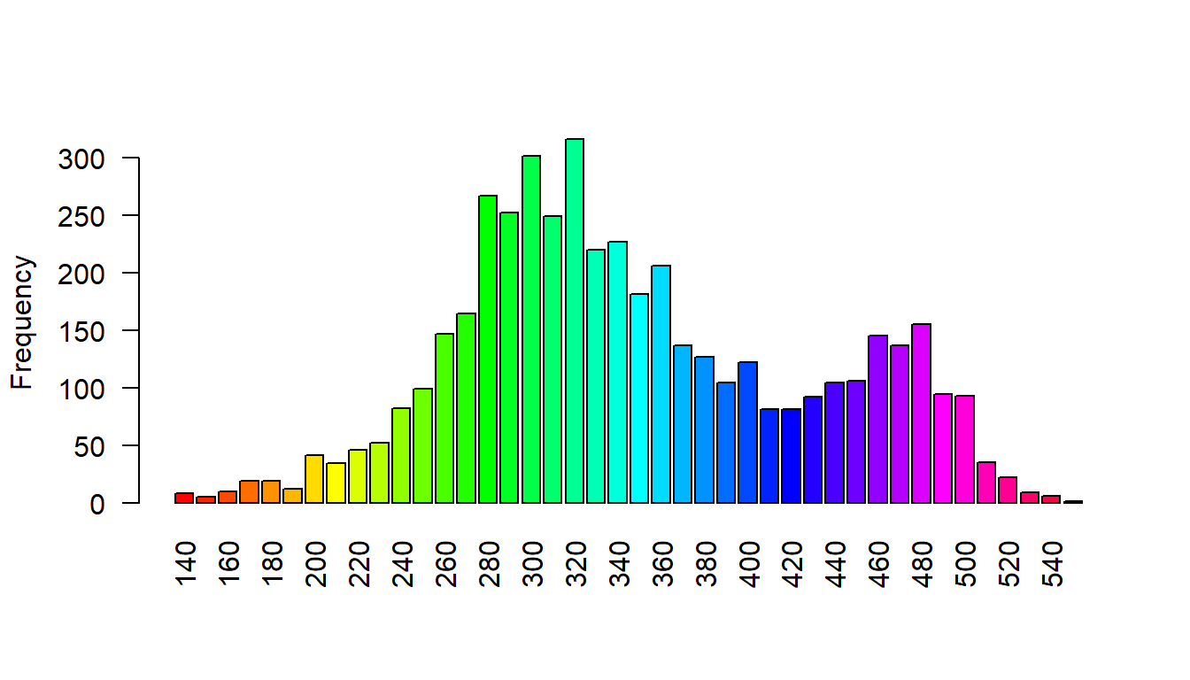

plot(elev)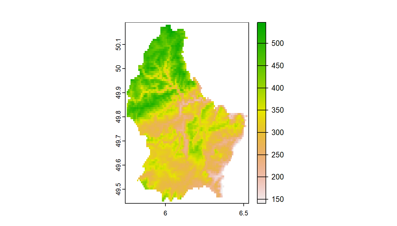

1.6.5 `stars` package

Load stock Landsat 7 .tif file that comes with package

tif = system.file("tif/L7_ETMs.tif", package = "stars")
read_stars(tif) |>
  dplyr::slice(index = 1, along = "band") |>
  plot()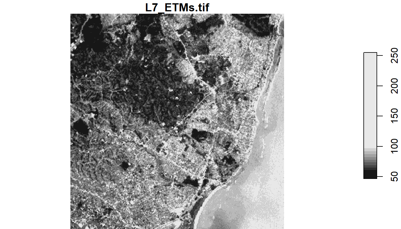

1.6.6 Convert flat files to spatial

We often have flat files, locally on our machine or accessed elsewhere, that have coordinate information which we would like to make spatial.

In the steps below, we

read in a .csv file of USGS gages in the PNW that have coordinate columns
Use st_as_sf function in sf to convert the data frame to an sf spatial simple feature collection by:
1. passing the coordinate columns to the coords parameter
2. specifying a coordinate reference system (CRS)
3. opting to retain the coordinate columns as attribute columns in the resulting sf feature collection.
Keep only the coordinates and station ID in resulting sf feature collection, and
Plotting our gages as spatial features with ggplot2 using geom_sf.

gages = read.csv(system.file("extdata/Gages_flowdata.csv", package = "Rspatialworkshop"))

gages_sf <- gages |> 
  st_as_sf(coords = c("LON_SITE", "LAT_SITE"), crs = 4269, remove = FALSE)  |> 
  dplyr::select(STATION_NM,LON_SITE, LAT_SITE)

ggplot() + geom_sf(data=gages_sf)

1.1 Goals and Outcomes

1.2 Background on data structures

1.2.1 Vectors

1.2.2 Atomic vectors

1.2.3 Matrix

1.2.4 Array

1.2.5 Lists

1.2.6 Data Frames

1.2.7 Data manipulation

1.2.8 Pipe operator

1.2.9 Filter

1.2.10 Select

1.2.11 Mutate

1.2.12 Summarize and Group_By

1.3 Why R for Spatial Data Analysis?

1.3.1 A Couple Motivating Examples

1.3.1.1 Choropleth map

1.3.1.2 Interactive mapping

1.4 Spatial Data Structures in R

1.4.1 Vector Data Model

1.4.1.1 Points

1.4.1.2 Lines

1.4.1.3 Polygon

1.4.1.4 Points, Lines, Polygons

1.4.1.5 Spatial Data Frames

1.4.2 Raster Data Model

1.4.2.1 Manipulating terra objects

1.4.2.2 Reading existing rasters on disk

1.4.3 Multiband rasters

1.4.3.1 Raster data with stars

1.5 Coordinate Reference Systems

1.5.1 The ellipsoid and geoid

1.5.2 Why you need to know about CRS working with spatial data in R:

1.5.3 Defining your coordinate reference system

1.5.4 Projected coordinate systems

1.5.5 Projecting

1.5.6 S2 class

1.6 Geographic Data Input/Output (I/O)

1.6.1 Reading in vector data

1.6.1.1 Shapefiles

1.6.1.2 Geodatabases

1.6.2 Geopackages

1.6.2.1 Open spatial data sources

1.6.2.2 Spatial data from R packages

1.6.2.3 Read in OpenStreetMap data

1.6.3 Reading in Raster data

1.6.4 terra package

1.6.5 stars package

1.6.6 Convert flat files to spatial

1.4.2.1 Manipulating `terra` objects

1.4.3.1 Raster data with `stars`

1.5.6 `S2` class

1.6.4 `terra` package

1.6.5 `stars` package