5  Additional Modeling Features

Throughout this section, we will use both the spmodel package and the ggplot2 package:

library(spmodel)
library(ggplot2)

We will continue to use the moss data throughout this section.

Goals:

• Incorporate additional arguments to splm() to:
  • Fit and predict for multiple models simultaneously.
  • Fit a spatial linear model with non-spatial random effects.
  • Fit a spatial linear model with anisotropy.
  • Fit a spatial linear model with a partition factor.
  • Fix certain spatial covariance parameters at known values.
  • Fit a random forest spatial residual linear model and make predictions.

5.1 Multiple Models

splm() fits multiple models simultaneously when spcov_type is a vector with more than one element:

spmods <- splm(formula = log_Zn ~ log_dist2road, data = moss,
              spcov_type = c("exponential", "gaussian"))

spmods is a list with two elements: exponential, using the exponential spatial covariance; and gaussian, using the Gaussian spatial covariance.

names(spmods)
#> [1] "exponential" "gaussian"

spmods is natural to combine with glances() to glance at each model fit:

glances(spmods)
#> # A tibble: 2 × 10
#>   model      n     p  npar value   AIC  AICc logLik deviance pseudo.r.squared
#>   <chr>  <int> <dbl> <int> <dbl> <dbl> <dbl>  <dbl>    <dbl>            <dbl>
#> 1 expon…   365     2     3  367.  373.  373.  -184.     363             0.683
#> 2 gauss…   365     2     3  435.  441.  441.  -218.     363.            0.686

and to combine with predict() to predict for each model fit.

Exercise

Work with a neighbor to find 90% confidence intervals for the fixed effects in the Gaussian model using either (1) tidy() or (2) confint(). Before beginning, decide with your neighbor who will begin working on (1) tidy() and who will begin working on (2) confint().

Exercise Solution

tidy(spmods$gaussian, conf.int = TRUE, conf.level = 0.90)
#> # A tibble: 2 × 7
#>   term          estimate std.error statistic p.value conf.low conf.high
#>   <chr>            <dbl>     <dbl>     <dbl>   <dbl>    <dbl>     <dbl>
#> 1 (Intercept)      9.21     0.196       46.9       0    8.89      9.53 
#> 2 log_dist2road   -0.519    0.0184     -28.2       0   -0.549    -0.489
confint(spmods$gaussian, level = 0.90)
#>                      5 %       95 %
#> (Intercept)    8.8853387  9.5310288
#> log_dist2road -0.5493091 -0.4887111

5.2 Non-Spatial Random Effects

In the moss data, there are actually some spatial locations that have more than one measurement due to multiple samples being collected at a single location or due to a single sample being tested multiple times in the laboratory. The sample variable indexes the spatial location:

moss
#> Simple feature collection with 365 features and 7 fields
#> Geometry type: POINT
#> Dimension:     XY
#> Bounding box:  xmin: -445884.1 ymin: 1929616 xmax: -383656.8 ymax: 2061414
#> Projected CRS: NAD83 / Alaska Albers
#> # A tibble: 365 × 8
#>   sample field_dup lab_rep year  sideroad log_dist2road log_Zn
#>   <fct>  <fct>     <fct>   <fct> <fct>            <dbl>  <dbl>
#> 1 001PR  1         1       2001  N                 2.68   7.33
#> 2 001PR  1         2       2001  N                 2.68   7.38
#> 3 002PR  1         1       2001  N                 2.54   7.58
#> 4 003PR  1         1       2001  N                 2.97   7.63
#> 5 004PR  1         1       2001  N                 2.72   7.26
#> 6 005PR  1         1       2001  N                 2.76   7.65
#> # ℹ 359 more rows
#> # ℹ 1 more variable: geometry <POINT [m]>

We might expect Zinc concentration to be correlated within a spatial location; therefore, we might want to add sample as a non-spatial random effect (here, an intercept random effect) to the model with log_Zn as the response and log_dist2road as the predictor. The splm() function allows non-spatial random effects to be incorporated with the random argument, which takes a formula specification that is similar in syntax as the nlme (Pinheiro and Bates 2006) and lme4 (Bates et al. 2015) packages.

randint <- splm(log_Zn ~ log_dist2road,
                data = moss, spcov_type = "exponential",
                random = ~ (1 | sample))

Tip

For the randint model, in the random argument, sample is shorthand for (1 | sample). So the randint model could be written more concisely as

randint <- splm(log_Zn ~ log_dist2road,
                      data = moss, spcov_type = "exponential",
                      random = ~ sample)

The summary output now shows an estimate of the variance of the random intercepts, in addition to the estimated fixed effects and estimated spatial covariance parameters.

summary(randint)
#> 
#> Call:
#> splm(formula = log_Zn ~ log_dist2road, data = moss, spcov_type = "exponential", 
#>     random = ~sample)
#> 
#> Residuals:
#>     Min      1Q  Median      3Q     Max 
#> -2.6234 -1.3228 -0.8026 -0.2642  1.0998 
#> 
#> Coefficients (fixed):
#>               Estimate Std. Error z value Pr(>|z|)    
#> (Intercept)    9.66066    0.26770   36.09   <2e-16 ***
#> log_dist2road -0.55028    0.02071  -26.58   <2e-16 ***
#> ---
#> Signif. codes:  0 '***' 0.001 '**' 0.01 '*' 0.05 '.' 0.1 ' ' 1
#> 
#> Pseudo R-squared: 0.6605
#> 
#> Coefficients (exponential spatial covariance):
#>        de        ie     range 
#> 3.153e-01 2.094e-02 1.083e+04 
#> 
#> Coefficients (random effects):
#> 1 | sample 
#>    0.07995

And, glances() shows that the model with the random intercepts is a better fit to the data than the model without random intercepts.

spmod <- splm(log_Zn ~ log_dist2road,
              data = moss, spcov_type = "exponential")
glances(spmod, randint)
#> # A tibble: 2 × 10
#>   model      n     p  npar value   AIC  AICc logLik deviance pseudo.r.squared
#>   <chr>  <int> <dbl> <int> <dbl> <dbl> <dbl>  <dbl>    <dbl>            <dbl>
#> 1 randi…   365     2     4  335.  343.  343.  -168.     363.            0.661
#> 2 spmod    365     2     3  367.  373.  373.  -184.     363             0.683

As another example, we might consider a model that also has random intercepts for year, or, a model that also has both random intercepts for year and random slopes for log_dist2road within year:

yearint <- splm(log_Zn ~ log_dist2road,
                      data = moss, spcov_type = "exponential",
                      random = ~ (1 | sample + year))
yearsl <- splm(log_Zn ~ log_dist2road,
                      data = moss, spcov_type = "exponential",
                      random = ~ (1 | sample) + 
                       (log_dist2road | year))

glances() shows that, of these four models, the model that includes random intercepts for sample, random intercepts for year, and random slopes for year is best, according to the AIC and AICc metrics.

glances(spmod, randint, yearint, yearsl)
#> # A tibble: 4 × 10
#>   model      n     p  npar value   AIC  AICc logLik deviance pseudo.r.squared
#>   <chr>  <int> <dbl> <int> <dbl> <dbl> <dbl>  <dbl>    <dbl>            <dbl>
#> 1 yearsl   365     2     6  190.  202.  202.  -94.9     363.            0.215
#> 2 yeari…   365     2     4  230.  238.  238. -115.      363.            0.729
#> 3 randi…   365     2     4  335.  343.  343. -168.      363.            0.661
#> 4 spmod    365     2     3  367.  373.  373. -184.      363             0.683

Note

The syntax ~ (log_dist2road | year) specifies that both random intercepts for year and random slopes for log_dist2road within year should be included in the model. If only random slopes are desired, then we should set random to ~ (-1 + log_dist2road | year).

Exercise

Perhaps a model with random intercepts for sample and random intercepts and slopes for year but without any spatial covariance is an even better fit to the data. Fit such a model by specifying spcov_type to be "none". Then, use glances() to see how well this non-spatial model fits the moss data compared to the spatially explicit models.

Exercise Solution

nospcov <- splm(log_Zn ~ log_dist2road,
                    data = moss, spcov_type = "none",
                    random = ~ (1 | sample) + 
                      (log_dist2road | year))
glances(spmod, randint, yearint, yearsl, nospcov)
#> # A tibble: 5 × 10
#>   model      n     p  npar value   AIC  AICc logLik deviance pseudo.r.squared
#>   <chr>  <int> <dbl> <int> <dbl> <dbl> <dbl>  <dbl>    <dbl>            <dbl>
#> 1 yearsl   365     2     6  190.  202.  202.  -94.9     363.            0.215
#> 2 yeari…   365     2     4  230.  238.  238. -115.      363.            0.729
#> 3 randi…   365     2     4  335.  343.  343. -168.      363.            0.661
#> 4 spmod    365     2     3  367.  373.  373. -184.      363             0.683
#> 5 nospc…   365     2     4  456.  464.  464. -228.      363             0.119
## the model with no explicit spatial covariance has the worst fit 
## of the five models.

5.3 Anisotropy

By default, splm() uses isotropic spatial covariance. Spatial covariance is isotropic if it behaves similarly in all directions. A spatial covariance is (geometrically) anisotropic if it does not behave similarly in all directions. Anisotropic models require estimation of two additional parameters: rotate and scale, which control the behavior of the spatial covariance as a function of distance and direction.

aniso <- splm(log_Zn ~ log_dist2road,
              data = moss, spcov_type = "exponential",
              anisotropy = TRUE)
aniso
#> 
#> Call:
#> splm(formula = log_Zn ~ log_dist2road, data = moss, spcov_type = "exponential", 
#>     anisotropy = TRUE)
#> 
#> 
#> Coefficients (fixed):
#>   (Intercept)  log_dist2road  
#>         9.548         -0.546  
#> 
#> 
#> Coefficients (exponential spatial covariance):
#>        de         ie      range     rotate      scale  
#> 3.561e-01  6.812e-02  8.732e+03  2.435e+00  4.753e-01

We can again use glances to compare the model that allows for anisotropy with the isotropic model:

glances(spmod, aniso)
#> # A tibble: 2 × 10
#>   model     n     p  npar value   AIC  AICc logLik deviance pseudo.r.squared
#>   <chr> <int> <dbl> <int> <dbl> <dbl> <dbl>  <dbl>    <dbl>            <dbl>
#> 1 aniso   365     2     5  362.  372.  372.  -181.     363.            0.705
#> 2 spmod   365     2     3  367.  373.  373.  -184.     363             0.683

The anisotropic model does have lower AIC and AICc than the isotropic model, indicating a better fit. However, the reduction in AIC and AICc is quite small, so we may still prefer the isotropic model for simplicity and interpretability.

Exercise

Visualize the anisotropic level curve for aniso using plot(). Hint: Run ?plot.spmodel or visit this link. Which direction does the model predict two responses will be more correlated?

Exercise Solution

plot(aniso, which = 8)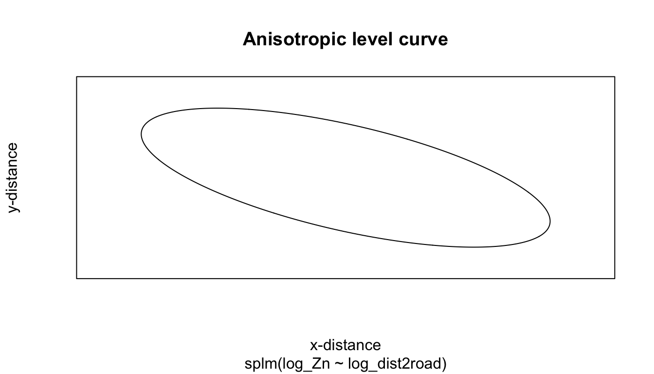

A clockwise rotation of this level curve by rotate followed by a scaling of the minor axis by the reciprocal of scale yields a spatial covariance that is isotropic.

5.4 Partition Factors

A partition factor is a categorical (or factor) variable that forces observations in different levels of the partition factor to be uncorrelated. The year variable in moss has two levels, 2001 and 2006, which correspond to the year of measurement. Suppose the goal is to fit a model that assumes observations from the same year are spatially correlated but observations from different years are not spatially correlated. In this context, year is a partition factor. We fit this model by running

part <- splm(log_Zn ~ log_dist2road,
             data = moss, spcov_type = "exponential",
             partition_factor = ~ year)

Like the formula and random arguments, the partition_factor argument requires a formula object.

5.5 Fixing Covariance Parameters

By default, splm() estimates all unknown covariance parameters. However, we can also fix covariance parameters at known values with the spcov_initial argument for spatial covariance parameters and with the randcov_initial argument for non-spatial covariance parameters.

As an example, suppose that we want to fit a "spherical" covariance model to the moss data, but that, we want to fix the range at 20000 units so that errors from spatial locations more than 20000 units apart are not spatially correlated. We first create an spcov_initial object with the spcov_initial() function:

init_spher <- spcov_initial("spherical", range = 20000, known = "range")
init_spher
#> $initial
#> range 
#> 20000 
#> 
#> $is_known
#> range 
#>  TRUE 
#> 
#> attr(,"class")
#> [1] "spherical"

Within the function call, we specify that, for a "spherical" covariance, we would like to set the range parameter to 20000 and for that value to be known and therefore fixed in any subsequent estimation. We then provide init_spher as an argument to spcov_initial in splm():

splm(log_Zn ~ log_dist2road, data = moss,
     spcov_initial = init_spher)
#> 
#> Call:
#> splm(formula = log_Zn ~ log_dist2road, data = moss, spcov_initial = init_spher)
#> 
#> 
#> Coefficients (fixed):
#>   (Intercept)  log_dist2road  
#>        9.7194        -0.5607  
#> 
#> 
#> Coefficients (spherical spatial covariance):
#>        de         ie      range  
#> 4.545e-01  8.572e-02  2.000e+04

When spcov_initial is provided, spcov_type is not a necessary argument to splm().

Exercise

Fit a "spherical" spatial covariance model to the moss data set without a nugget effect (i.e., the model should have the ie independent variance parameter set to 0 and treated as known). Verify in the summary output that the ie is indeed 0 for this model.

Exercise Solution

init_no_ie <- spcov_initial("spherical", ie = 0, known = "ie")
no_ie <- splm(log_Zn ~ log_dist2road, data = moss,
              spcov_initial = init_no_ie)
summary(no_ie)
#> 
#> Call:
#> splm(formula = log_Zn ~ log_dist2road, data = moss, spcov_initial = init_no_ie)
#> 
#> Residuals:
#>     Min      1Q  Median      3Q     Max 
#> -3.1766 -1.8420 -1.2975 -0.7249  0.6577 
#> 
#> Coefficients (fixed):
#>               Estimate Std. Error z value Pr(>|z|)    
#> (Intercept)   10.27912   28.99660   0.354    0.723    
#> log_dist2road -0.56642    0.01974 -28.693   <2e-16 ***
#> ---
#> Signif. codes:  0 '***' 0.001 '**' 0.01 '*' 0.05 '.' 0.1 ' ' 1
#> 
#> Pseudo R-squared: 0.6967
#> 
#> Coefficients (spherical spatial covariance):
#>        de        ie     range 
#> 8.433e+02 0.000e+00 3.699e+07

5.6 Random Forest Spatial Residual Models

Random forests are a popular machine-learning modeling tool. The random forest spatial residual model available in spmodel combines random forest modeling and spatial linear models. First, the model is fit using random forests and fitted values are obtained. Then the response residuals are used to fit a spatial linear model. Predictions at unobserved locations are computed as the sum of the random forest prediction and the predicted (i.e., Kriged) response residual from the spatial linear model. Suppose we split the moss data into training and test data sets, with the goal of predicting log_Zn in the test data.

set.seed(1)
n <- NROW(moss)
n_train <- round(0.75 * n)
n_test <- n - n_train
train_index <- sample(n, size = n_train)
moss_train <- moss[train_index, , ]
moss_test <- moss[-train_index, , ]

We fit a random forest spatial residual model to the test data by running

rfsrmod <- splmRF(log_Zn ~ log_dist2road, moss_train,
                  spcov_type = "exponential")

We make predictions for the test data by running

# results omitted
predict(rfsrmod, moss_test)

Exercise

Use predict() to store the random forest spatial residual predictions of log_Zn at locations in the test data and then compute the mean-squared prediction error.

Exercise Solution

preds <- predict(rfsrmod, newdata = moss_test)
errors <- moss_test$log_Zn - preds
mean(errors^2)
#> [1] 0.1831002

5.7 R Code Appendix

library(spmodel)
library(ggplot2)
spmods <- splm(formula = log_Zn ~ log_dist2road, data = moss,
              spcov_type = c("exponential", "gaussian"))
names(spmods)
glances(spmods)
tidy(spmods$gaussian, conf.int = TRUE, conf.level = 0.90)
confint(spmods$gaussian, level = 0.90)
moss
randint <- splm(log_Zn ~ log_dist2road,
                data = moss, spcov_type = "exponential",
                random = ~ (1 | sample))
randint <- splm(log_Zn ~ log_dist2road,
                      data = moss, spcov_type = "exponential",
                      random = ~ sample)
summary(randint)
spmod <- splm(log_Zn ~ log_dist2road,
              data = moss, spcov_type = "exponential")
glances(spmod, randint)
yearint <- splm(log_Zn ~ log_dist2road,
                      data = moss, spcov_type = "exponential",
                      random = ~ (1 | sample + year))
yearsl <- splm(log_Zn ~ log_dist2road,
                      data = moss, spcov_type = "exponential",
                      random = ~ (1 | sample) + 
                       (log_dist2road | year))
glances(spmod, randint, yearint, yearsl)
nospcov <- splm(log_Zn ~ log_dist2road,
                    data = moss, spcov_type = "none",
                    random = ~ (1 | sample) + 
                      (log_dist2road | year))
glances(spmod, randint, yearint, yearsl, nospcov)
## the model with no explicit spatial covariance has the worst fit 
## of the five models.
aniso <- splm(log_Zn ~ log_dist2road,
              data = moss, spcov_type = "exponential",
              anisotropy = TRUE)
aniso
glances(spmod, aniso)
plot(aniso, which = 8)
part <- splm(log_Zn ~ log_dist2road,
             data = moss, spcov_type = "exponential",
             partition_factor = ~ year)
init_spher <- spcov_initial("spherical", range = 20000, known = "range")
init_spher
splm(log_Zn ~ log_dist2road, data = moss,
     spcov_initial = init_spher)
init_no_ie <- spcov_initial("spherical", ie = 0, known = "ie")
no_ie <- splm(log_Zn ~ log_dist2road, data = moss,
              spcov_initial = init_no_ie)
summary(no_ie)
set.seed(1)
n <- NROW(moss)
n_train <- round(0.75 * n)
n_test <- n - n_train
train_index <- sample(n, size = n_train)
moss_train <- moss[train_index, , ]
moss_test <- moss[-train_index, , ]
rfsrmod <- splmRF(log_Zn ~ log_dist2road, moss_train,
                  spcov_type = "exponential")
# results omitted
predict(rfsrmod, moss_test)
preds <- predict(rfsrmod, newdata = moss_test)
errors <- moss_test$log_Zn - preds
mean(errors^2)

Bates, Douglas, Martin Mächler, Ben Bolker, and Steve Walker. 2015. “Fitting Linear Mixed-Effects Models Using lme4.” Journal of Statistical Software 67 (1): 1–48. https://doi.org/10.18637/jss.v067.i01.

Pinheiro, José, and Douglas Bates. 2006. Mixed-Effects Models in S and S-PLUS. Springer science & business media.