3  Model Fitting

Throughout this section, we will use both the spmodel package and the ggplot2 package:

library(spmodel)
library(ggplot2)

Goals:

• Further explore the splm() function using the moss data.
• Connect parameter estimates in the summary output of splm() to the spatial linear model.

3.1 Data Introduction

The moss data in the spmodel package is an sf (simple features) object (Pebesma 2018) that contains observations on heavy metals in mosses near a mining road in Alaska. An sf object is a special data.frame built for storing spatial information and contains a column called geometry. We can view the first few rows of moss by running

moss
#> Simple feature collection with 365 features and 7 fields
#> Geometry type: POINT
#> Dimension:     XY
#> Bounding box:  xmin: -445884.1 ymin: 1929616 xmax: -383656.8 ymax: 2061414
#> Projected CRS: NAD83 / Alaska Albers
#> # A tibble: 365 × 8
#>   sample field_dup lab_rep year  sideroad log_dist2road log_Zn
#>   <fct>  <fct>     <fct>   <fct> <fct>            <dbl>  <dbl>
#> 1 001PR  1         1       2001  N                 2.68   7.33
#> 2 001PR  1         2       2001  N                 2.68   7.38
#> 3 002PR  1         1       2001  N                 2.54   7.58
#> 4 003PR  1         1       2001  N                 2.97   7.63
#> 5 004PR  1         1       2001  N                 2.72   7.26
#> 6 005PR  1         1       2001  N                 2.76   7.65
#> # ℹ 359 more rows
#> # ℹ 1 more variable: geometry <POINT [m]>

More information about moss can be found by running help("moss", "spmodel").

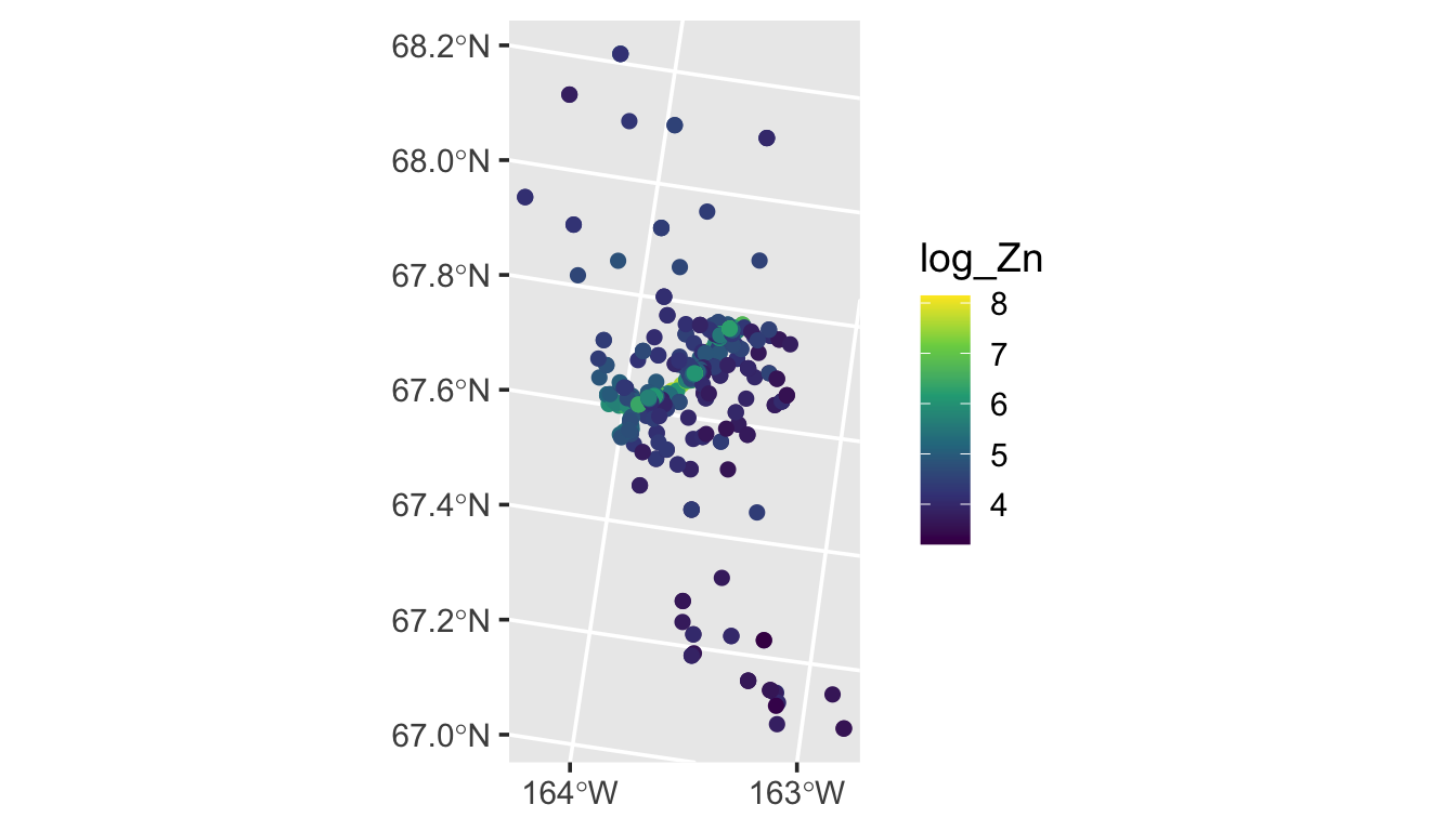
Our goal is to model the distribution of log zinc concentration (log_Zn) using a spatial linear model. We can visualize the distribution of log zinc concentration (log_Zn) in moss by running

ggplot(moss, aes(color = log_Zn)) +
  geom_sf(size = 2) +
  scale_color_viridis_c() +
  scale_x_continuous(breaks = seq(-163, -164, length.out = 2)) +
  theme_gray(base_size = 14)

Distribution of log zinc concentration in the moss data.

An important predictor variable may be the log of the distance to the haul road, log_dist2road, which is measured in meters. Next we use spmodel to fit a spatial linear model with with log_Zn as the response and log_dist2road as a predictor.

3.2 splm() Syntax and Output Interpretation

The splm() function shares similar syntactic structure with the lm() function used to fit linear models without spatial dependence (Equation 2.1). splm() generally requires at least three arguments

• formula: a formula that describes the relationship between the response variable (\(\mathbf{y}\)) and explanatory variables (\(\mathbf{X}\))
  • formula in splm() is the same as formula in lm()
• data: a data.frame or sf object that contains the response variable, explanatory variables, and spatial information.
• spcov_type: the spatial covariance type ("exponential", "matern", "spherical", etc)
  • There are 17 different types

Note

If data is an sf object, then spatial information is stored in the object’s geometry. However, if data is a data.frame or tibble (a special data.frame), then the names of the variables that represent the x-coordinates and y-coordinates must also be provided as two additional arguments via xcoord and ycoord.

We fit a spatial linear model regressing log zinc concentration (log_Zn) on log distance to a haul road (log_dist2road) using an exponential spatial covariance function by running

spmod <- splm(formula = log_Zn ~ log_dist2road, data = moss,
              spcov_type = "exponential")

Tip

The estimation method in splm() is specified by estmethod. The default estimation method is restricted maximum likelihood ("reml"). Additional options include maximum likelihood "ml", semivariogram-based composite likelihood ("sv-cl") (Curriero and Lele 1999), and semivariogram-based weighted least squares ("sv-wls") (Cressie 1985). When the estimation method is semivariogram-based weighted least squares, the weights are specified by weights with a default of Cressie weights (“cressie").

We summarize the model fit by running

summary(spmod)
#> 
#> Call:
#> splm(formula = log_Zn ~ log_dist2road, data = moss, spcov_type = "exponential")
#> 
#> Residuals:
#>     Min      1Q  Median      3Q     Max 
#> -2.6801 -1.3606 -0.8103 -0.2485  1.1298 
#> 
#> Coefficients (fixed):
#>               Estimate Std. Error z value Pr(>|z|)    
#> (Intercept)    9.76825    0.25216   38.74   <2e-16 ***
#> log_dist2road -0.56287    0.02013  -27.96   <2e-16 ***
#> ---
#> Signif. codes:  0 '***' 0.001 '**' 0.01 '*' 0.05 '.' 0.1 ' ' 1
#> 
#> Pseudo R-squared: 0.683
#> 
#> Coefficients (exponential spatial covariance):
#>        de        ie     range 
#> 3.595e-01 7.897e-02 8.237e+03

The fixed effects coefficient table contains estimates, standard errors, z-statistics, and asymptotic p-values for each fixed effect. From this table, we notice there is evidence that mean log zinc concentration significantly decreases with distance from the haul road (p-value < 2e-16).

We can relate some of the components in the summary output to the model in Equation 2.2:

• The values in the Estimate column of the Coefficients (fixed) table form \(\boldsymbol{\hat{\beta}}\), an estimate of \(\boldsymbol{\beta}\).
• The de value of 0.36 in the Coefficients (exponential spatial covariance) table is \(\hat{\sigma}^2_{de}\), which is an estimate of \(\sigma^2_{de}\), the variance of \(\boldsymbol{\tau}\) (commonly called the partial sill).
• The ie value of 0.079 in the Coefficients (exponential spatial covariance) table is \(\hat{\sigma}^2_{ie}\), which is an estimate of \(\sigma^2_{ie}\), the variance of \(\boldsymbol{\epsilon}\) (commonly called the nugget).
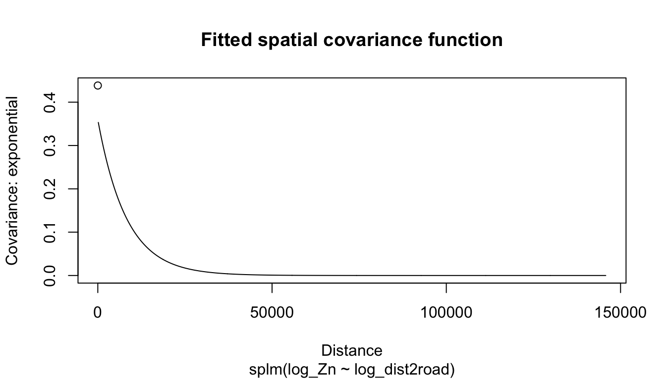
• The range value of 8,237 in the Coefficients (exponential spatial covariance) table is \(\hat{\phi}\), which is an estimate of \(\phi\) (recall \(\phi\) is the range parameter in Equation 2.3 that controls the behavior of the spatial covariance as a function of distance).

The summary() output, while useful, is printed to the R console and not easy to manipulate. The tidy() function turns the coefficient table into a tibble (i.e., a special data.frame) that is easy to manipulate. We tidy the fixed effects by running

tidy(spmod)
#> # A tibble: 2 × 5
#>   term          estimate std.error statistic p.value
#>   <chr>            <dbl>     <dbl>     <dbl>   <dbl>
#> 1 (Intercept)      9.77     0.252       38.7       0
#> 2 log_dist2road   -0.563    0.0201     -28.0       0

We tidy the spatial covariance parameters by running

tidy(spmod, effects = "spcov")
#> # A tibble: 3 × 3
#>   term   estimate is_known
#>   <chr>     <dbl> <lgl>   
#> 1 de       0.360  FALSE   
#> 2 ie       0.0790 FALSE   
#> 3 range 8237.     FALSE

The is_known column indicates whether the parameter is assumed known. By default, all parameters are assumed unknown. We discuss this more in Chapter 5.

Exercise

Another data set contained within the spmodel package is the caribou data set. Read about the caribou data with ?caribou. Then, fit a spatial linear model with

• z as the response and tarp, water, and the interaction between tarp and water as predictors
• a spatial covariance model for the errors of your choosing. You can examine the spatial covariance models available to use in the spcov_type argument of splm() in the Arguments section of ?splm.
• x as the xcoord and y as the ycoord (note that the xcoord and ycoord arguments now need to be specified because caribou is a data.frame object, not an sf object).

After fitting the model, perform an analysis of variance using anova() to assess the importance of tarp, water, and tarp:water.

Solution

caribou_mod <- splm(z ~ tarp + water + tarp:water,
                    data = caribou, spcov_type = "pexponential",
                    xcoord = x, ycoord = y)
summary(caribou_mod)
#> 
#> Call:
#> splm(formula = z ~ tarp + water + tarp:water, data = caribou, 
#>     spcov_type = "pexponential", xcoord = x, ycoord = y)
#> 
#> Residuals:
#>      Min       1Q   Median       3Q      Max 
#> -0.35291 -0.20863 -0.14249 -0.01117  0.38358 
#> 
#> Coefficients (fixed):
#>                  Estimate Std. Error z value Pr(>|z|)    
#> (Intercept)       1.98991    3.69849   0.538 0.590555    
#> tarpnone          0.17267    0.10645   1.622 0.104790    
#> tarpshade         0.39551    0.10471   3.777 0.000159 ***
#> waterY            0.04751    0.10394   0.457 0.647570    
#> tarpnone:waterY  -0.18487    0.14778  -1.251 0.210919    
#> tarpshade:waterY -0.21760    0.14463  -1.505 0.132437    
#> ---
#> Signif. codes:  0 '***' 0.001 '**' 0.01 '*' 0.05 '.' 0.1 ' ' 1
#> 
#> Pseudo R-squared: 0.4559
#> 
#> Coefficients (pexponential spatial covariance):
#>        de        ie     range     extra 
#>   13.6922    0.0215 2257.4371    0.9125
anova(caribou_mod)
#> Analysis of Variance Table
#> 
#> Response: z
#>             Df    Chi2 Pr(>Chi2)    
#> (Intercept)  1  0.2895 0.5905550    
#> tarp         2 14.4455 0.0007298 ***
#> water        1  0.2090 0.6475699    
#> tarp:water   2  2.5913 0.2737193    
#> ---
#> Signif. codes:  0 '***' 0.001 '**' 0.01 '*' 0.05 '.' 0.1 ' ' 1
tidy(anova(caribou_mod))
#> # A tibble: 4 × 4
#>   effects        df statistic  p.value
#>   <chr>       <int>     <dbl>    <dbl>
#> 1 (Intercept)     1     0.289 0.591   
#> 2 tarp            2    14.4   0.000730
#> 3 water           1     0.209 0.648   
#> 4 tarp:water      2     2.59  0.274

3.3 Model Fit and Diagnostics

The quality of model fit can be assessed using a variety of statistics readily available in spmodel, including AIC, AICc, and pseudo R-squared. Additionally, model diagnostics such as leverage, fitted values, residuals (several types), and Cook’s distance. While both the model fit statistics and the diagnostics can be found with individual functions like AIC(), residuals(), cooks.distance(), etc., they can also be computed using glance() (for the model fit statistics) and augment() (for the diagnostics).

glance(spmod)
#> # A tibble: 1 × 9
#>       n     p  npar value   AIC  AICc logLik deviance pseudo.r.squared
#>   <int> <dbl> <int> <dbl> <dbl> <dbl>  <dbl>    <dbl>            <dbl>
#> 1   365     2     3  367.  373.  373.  -184.      363            0.683

The output from glance() shows model fit statistics for the spatial linear model with an exponential covariance structure for the errors.

Exercise

The glances() function allows us to compare the model fit statistics for a few different models simultaneously. Use splm() to fit a model with a Matérn spatial covariance (by specifying "matern" for spcov_type) and a model with no spatial covariance (by specifying "none" for spcov_type). Then, use the glances() function, providing each model object as an argument, to compare the model fit statistics of each model.

Solution

mat <- splm(formula = log_Zn ~ log_dist2road, data = moss,
              spcov_type = "matern")
none <- splm(formula = log_Zn ~ log_dist2road, data = moss,
              spcov_type = "none")
glances(spmod, mat, none)
#> # A tibble: 3 × 10
#>   model     n     p  npar value   AIC  AICc logLik deviance pseudo.r.squared
#>   <chr> <int> <dbl> <int> <dbl> <dbl> <dbl>  <dbl>    <dbl>            <dbl>
#> 1 mat     365     2     4  316.  324.  324.  -158.     363             0.630
#> 2 spmod   365     2     3  367.  373.  373.  -184.     363             0.683
#> 3 none    365     2     1  634.  636.  636.  -317.     363.            0.671

We see from the output that (1) the spatial models provide a much better fit to the data than the linear model with independent errors and (2) the extra “smoothness” parameter incorporated in the "matern" covariance substantially improves the model fit compared to the "exponential" covariance. We are able to tell this by looking at the AICc, which glances() automatically sorts by (lower values of AIC and AICc indicate a better model fit).

The augment() function provides many model diagnostics statistics in a single tibble:

augment(spmod)
#> Simple feature collection with 365 features and 7 fields
#> Geometry type: POINT
#> Dimension:     XY
#> Bounding box:  xmin: -445884.1 ymin: 1929616 xmax: -383656.8 ymax: 2061414
#> Projected CRS: NAD83 / Alaska Albers
#> # A tibble: 365 × 8
#>   log_Zn log_dist2road .fitted .resid   .hat .cooksd .std.resid
#> *  <dbl>         <dbl>   <dbl>  <dbl>  <dbl>   <dbl>      <dbl>
#> 1   7.33          2.68    8.26 -0.928 0.0200 0.0142       1.18 
#> 2   7.38          2.68    8.26 -0.880 0.0200 0.0186       1.35 
#> 3   7.58          2.54    8.34 -0.755 0.0225 0.00482      0.647
#> 4   7.63          2.97    8.09 -0.464 0.0197 0.0305       1.74 
#> 5   7.26          2.72    8.24 -0.977 0.0215 0.131        3.45 
#> 6   7.65          2.76    8.21 -0.568 0.0284 0.0521       1.89 
#> # ℹ 359 more rows
#> # ℹ 1 more variable: geometry <POINT [m]>

augment() returns a tibble with many model diagnostics statistics, including

• .fitted, the fitted value, calculated from the estimated fixed effects in the model
• .hat, the Mahalanobis distance, a metric of leverage
• .cooksd, the Cook’s distance, a metric of influence
• .std.resid, the standardized residual

If the model is correct, then the standardized residuals have mean 0, standard deviation 1, and are uncorrelated.

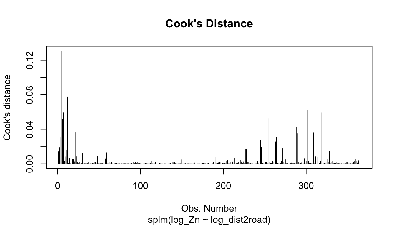
The plot() function can be used on a fitted model object to construct a few pre-specified plots of these model diagnostics. For example, the following code plots the Cook’s distance, a measure of influence, which quantifies each observation’s impact on model fit:

plot(spmod, which = 4)

The other 7 plots for model objects fit with splm() can be read about in the help: ?plot.spmodel.

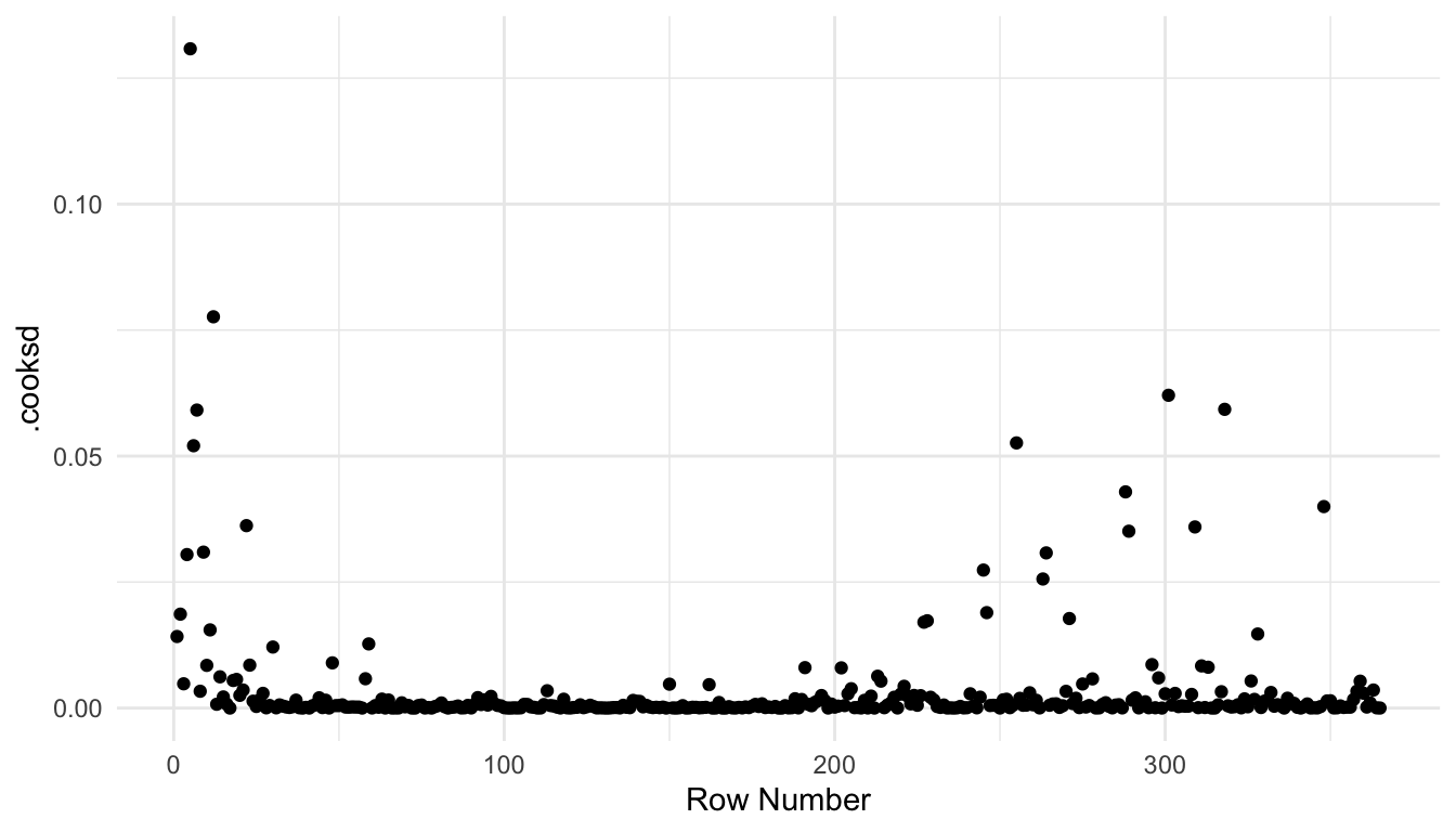
If the grammar of graphics plotting syntax in ggplot2 is more familiar, then we can also construct plots with the augmented model:

aug_df <- augment(spmod)
ggplot(data = aug_df, aes(x = seq_len(nrow(aug_df)),
                          y = .cooksd)) +
  geom_point() +
  theme_minimal() +
  labs(x = "Row Number")

Exercise

Use spmodel’s plot function on the spmod object to construct a plot of the fitted spatial covariance vs spatial distance. To learn more about the options for spmodel’s plot function, run ?plot.spmodel or visit this link.

Solution

plot(spmod, which = 7)

3.4 R Code Appendix

library(spmodel)
library(ggplot2)
moss
ggplot(moss, aes(color = log_Zn)) +
  geom_sf(size = 2) +
  scale_color_viridis_c() +
  scale_x_continuous(breaks = seq(-163, -164, length.out = 2)) +
  theme_gray(base_size = 14)
spmod <- splm(formula = log_Zn ~ log_dist2road, data = moss,
              spcov_type = "exponential")
summary(spmod)
tidy(spmod)
tidy(spmod, effects = "spcov")
caribou_mod <- splm(z ~ tarp + water + tarp:water,
                    data = caribou, spcov_type = "pexponential",
                    xcoord = x, ycoord = y)
summary(caribou_mod)
anova(caribou_mod)
tidy(anova(caribou_mod))
glance(spmod)
mat <- splm(formula = log_Zn ~ log_dist2road, data = moss,
              spcov_type = "matern")
none <- splm(formula = log_Zn ~ log_dist2road, data = moss,
              spcov_type = "none")
glances(spmod, mat, none)
augment(spmod)
plot(spmod, which = 4)
aug_df <- augment(spmod)
ggplot(data = aug_df, aes(x = seq_len(nrow(aug_df)),
                          y = .cooksd)) +
  geom_point() +
  theme_minimal() +
  labs(x = "Row Number")
plot(spmod, which = 7)

Cressie, Noel. 1985. “Fitting Variogram Models by Weighted Least Squares.” Journal of the International Association for Mathematical Geology 17 (5): 563–86.

Curriero, Frank C, and Subhash Lele. 1999. “A Composite Likelihood Approach to Semivariogram Estimation.” Journal of Agricultural, Biological, and Environmental Statistics, 9–28.

Pebesma, Edzer. 2018. “Simple Features for R: Standardized Support for Spatial Vector Data.” The R Journal 10 (1): 439–46. https://doi.org/10.32614/RJ-2018-009.