Spatial Generalized Linear Models in spmodel

Introduction

spmodel is an R package used to fit, summarize, and predict for a variety of spatial statistical models. The vignette provides an introduction spatial generalized linear models for non-Gaussian response distributions in spmodel. Before proceeding, we load spmodel by running

library(spmodel)

If using spmodel in a formal publication or report, please cite it. Citing spmodel lets us devote more resources to the package in the future. We view the spmodel citation by running

citation(package = "spmodel")

#> To cite spmodel in publications use:
#> 
#>   Dumelle M, Higham M, Ver Hoef JM (2023). spmodel: Spatial statistical
#>   modeling and prediction in R. PLOS ONE 18(3): e0282524.
#>   https://doi.org/10.1371/journal.pone.0282524
#> 
#> A BibTeX entry for LaTeX users is
#> 
#>   @Article{,
#>     title = {{spmodel}: Spatial statistical modeling and prediction in {R}},
#>     author = {Michael Dumelle and Matt Higham and Jay M. {Ver Hoef}},
#>     journal = {PLOS ONE},
#>     year = {2023},
#>     volume = {18},
#>     number = {3},
#>     pages = {1--32},
#>     doi = {10.1371/journal.pone.0282524},
#>     url = {https://doi.org/10.1371/journal.pone.0282524},
#>   }

We will create visualizations using ggplot2 (Wickham 2016), which we load by running

library(ggplot2)

ggplot2 is only installed alongside spmodel when dependencies = TRUE in install.packages(), so check that the package is installed and loaded before reproducing any of these vignette’s visualizations. We will also show code that can be used to create interactive visualizations of spatial data with mapview (Appelhans et al. 2022). mapview also has many backgrounds available that contextualize spatial data with topographical information. Before running the mapview code interactively, make sure mapview is installed and loaded.

spmodel contains various methods for generic functions defined outside of spmodel. To find relevant documentation for these methods, run help("generic.spmodel", "spmodel") (e.g., help("summary.spmodel", "spmodel"), help("predict.spmodel", "spmodel"), etc.). Note that ?generic.spmodel is shorthand for help("generic.spmodel", "spmodel"). We provide more details and examples regarding these methods and generics throughout this vignette. For a full list of spmodel functions available, see spmodel’s documentation manual.

A Review of the Spatial Linear Model

We first focus on spatial linear models for a Gaussian response vector. The spatial linear model is defined as \[\begin{equation}\label{eq:splm} \mathbf{y} = \mathbf{X} \boldsymbol{\beta} + \boldsymbol{\tau} + \boldsymbol{\epsilon}, \end{equation}\] where for a sample size \(n\), \(\mathbf{y}\) is an \(n \times 1\) column vector of response variables, \(\mathbf{X}\) is an \(n \times p\) design (model) matrix of explanatory variables, \(\boldsymbol{\beta}\) is a \(p \times 1\) column vector of fixed effects controlling the impact of \(\mathbf{X}\) on \(\mathbf{y}\), \(\boldsymbol{\tau}\) is an \(n \times 1\) column vector of spatially dependent random errors, and \(\boldsymbol{\epsilon}\) is an \(n \times 1\) column vector of spatially independent random errors. We make a few assumptions about \(\boldsymbol{\tau}\) and \(\boldsymbol{\epsilon}\) in the spatial linear model: first, that \(\text{E}(\boldsymbol{\tau}) = \text{E}(\boldsymbol{\epsilon}) = \boldsymbol{0}\), where \(\text{E}(\cdot)\) denotes expectation; second, that \(\text{Cov}(\boldsymbol{\tau}) = \sigma^2_\tau \mathbf{R}\), where \(\mathbf{R}\) is an \(n \times n\) matrix that determines the spatial dependence structure in \(\mathbf{y}\) and depends on a range parameter, \(\phi\); third, that \(\text{Cov}(\boldsymbol{\epsilon}) = \sigma^2_\epsilon \mathbf{I}\), where \(\mathbf{I}\) is an \(n \times n\) identity matrix; and fourth, that \(\boldsymbol{\tau}\) and \(\boldsymbol{\epsilon}\) are independent of one another. The parameter \(\sigma^2_{\tau}\) is called the spatially dependent random error variance or partial sill. The parameter \(\sigma^2_\epsilon\) is called the spatially independent random error variance or nugget. These two variance parameters are henceforth more intuitively written as \(\sigma^2_{de}\) and \(\sigma^2_{ie}\), respectively. The covariance of \(\mathbf{y}\) is denoted \(\boldsymbol{\Sigma}\) and given by \[\begin{equation}\label{eq:spcov} \boldsymbol{\Sigma} = \sigma^2_{de}\mathbf{R} + \sigma^2_{ie} \mathbf{I}. \end{equation}\] The parameters \(\sigma^2_{de}\), \(\phi\), and \(\sigma^2_{ie}\) are elements of \(\boldsymbol{\theta}\), the covariance parameter vector.

The spatial linear model applies to both point-referenced and areal (i.e., lattice; polygon) data. Spatial data are point-referenced when the elements in \(\mathbf{y}\) are observed at point-locations indexed by x-coordinates and y-coordinates on a spatially continuous surface with an infinite number of locations. For example, consider sampling soil at any point-location in a field. Spatial linear models for point-referenced data are sometimes called geostatistical models. An example of an \(\mathbf{R}\) matrix for point-referenced data is the spherical correlation matrix given by \[\begin{equation}\label{eq:spherical} \mathbf{R} = \left(1 - 1.5\frac{\mathbf{H}}{\phi} + 0.5\frac{\mathbf{H}^3}{\phi^3}\right) \odot \mathcal{I}(\mathbf{H} \leq \phi), \end{equation}\]
where \(\mathbf{H}\) is a matrix of Euclidean distances among observations, \(\mathbf{H}^3\) is a matrix of cubed Euclidean distances, \(\odot\) is the Hadmard (element-wise; direct) product, and \(\mathcal{I}(\mathbf{H} \leq \phi)\) is an indicator function equal to one when the \(ij\)th element of \(\mathbf{H}\) is less than \(\phi\) (the range) and zero otherwise. A second is example is the Matérn correlation matrix given by \[\begin{equation}\label{eq:matern} \mathbf{R} = \frac{2^{1 - \nu}}{\Gamma(\nu)} \left(2\nu \mathbf{H} / \phi \right)^{\nu / 2} \odot B_k(2\nu \mathbf{H}, \nu), \end{equation}\] where \(\nu\) is a smoothness parameter, \(\odot\) is the Hadmart (element-wise; direct) product, and \(B_k(\cdot, \nu)\) is a Bessel-K function with order \(\nu\). Chiles and Delfiner (2012) provide examples of several spatial dependence structures.

Spatial data are areal when they are observed as part of a finite network of polygons whose connections are indexed by a neighborhood structure. For example, the polygons may represent counties in a state who are neighbors if they share at least one boundary. An example of an \(\mathbf{R}\) matrix for areal data is the simultaneous-autoregressive spatial correlation matrix given by \[\begin{equation*} \mathbf{R} = [(\mathbf{I} - \phi \mathbf{W})(\mathbf{I} - \phi \mathbf{W})^\top]^{-1}, \end{equation*}\] where \(\mathbf{W}\) is a weight matrix that describes the neighborhood structure among observations. Spatial linear models for areal data are sometimes called spatial autoregressive models. For thorough reviews of the spatial linear model, see Cressie (1993), Banerjee, Carlin, and Gelfand (2014), and Schabenberger and Gotway (2017).

The Spatial Generalized Linear Model

It is common to implicitly assume \(\mathbf{y}\) in the spatial linear model is unconstrained and Gaussian. This is a restrictive assumption and often inappropriate for binary data, proportion data, count data, and skewed data, which are common in many practical applications. These types of data are most naturally described using generalized linear models (Nelder and Wedderburn 1972; McCullagh and Nelder 1989). Generalized linear models are an extension of linear models that “link” a function of a distribution’s mean to the linear function \(\mathbf{X} \boldsymbol{\beta}\) (the explanatory variables and fixed effects). We can extend generalized linear models by adding linear, latent (i.e., unobserved) random effects to \(\mathbf{X} \boldsymbol{\beta}\). These types of models are called generalized linear mixed models (Breslow and Clayton 1993) and are often formulated using a hierarchical construction (Lee and Nelder 1996). For thorough reviews of generalized linear models and generalized linear mixed models, see Bolker et al. (2009), Myers et al. (2012), Faraway (2016), and Wood (2017).

A recent spmodel release (version 0.4.0) provided support for spatial generalized linear models (i.e., a generalized linear mixed model with spatial random effects). We define the spatial generalized linear model as \[\begin{equation}\label{eq:spglm} f(\boldsymbol{\mu}) \equiv \mathbf{w} = \mathbf{X} \boldsymbol{\beta} + \boldsymbol{\tau} + \boldsymbol{\epsilon}, \end{equation}\] where \(f(\cdot)\) is the link function, \(\boldsymbol{\mu}\) is the mean of \(\mathbf{y}\), and the remaining terms \(\mathbf{X}\), \(\boldsymbol{\beta}\), \(\boldsymbol{\tau}\), \(\boldsymbol{\epsilon}\) represent the same quantities as for spatial linear models. That is, \(\text{E}(\boldsymbol{\tau}) = \text{E}(\boldsymbol{\epsilon}) = \boldsymbol{0}\), \(\text{Cov}(\boldsymbol{\tau}) = \sigma^2_{de}\mathbf{R}\), \(\text{Cov}(\boldsymbol{\epsilon}) = \sigma^2_{ie} \mathbf{I}\), \(\boldsymbol{\tau}\) is independent of \(\boldsymbol{\epsilon}\), and \(\boldsymbol{\Sigma} = \sigma^2_{de} \mathbf{R} + \sigma^2_{ie} \mathbf{I}\). The link function, \(f(\cdot)\), “links” a function of \(\boldsymbol{\mu}\) to the linear term \(\mathbf{w}\). Note that the linking of \(\boldsymbol{\mu}\) to \(\mathbf{w}\) applies element-wise to each vector. Each link function \(f(\cdot)\) has a corresponding inverse link function, \(f^{-1}(\cdot)\), which “links” a function of \(\mathbf{w}\) to \(\boldsymbol{\mu}\). Notice that \(\mathbf{w}\) is unconstrained but \(\boldsymbol{\mu}\) is usually constrained in some way (e.g., positive) that depends on the distribution assumed for \(\mathbf{y}\).

Spatial linear and generalized linear models rely on the same components: explanatory variables, fixed effects, spatially dependent random errors, and spatial independent random errors. These components are related to the response linearly (spatial linear models) or non-linearly (spatial generalized linear models). The response itself is generally assumed to follow a Gaussian distribution (spatial linear models) or one of many non-Gaussian distributions (spatial generalized linear models). Some non-Gaussian distributions include the binomial distribution for binary responses, the beta distribution for proportion responses, the Poisson or negative binomial distributions for count responses, and the gamma or inverse Gaussian distributions for skewed, positive continuous responses.

spmodel implements a marginal approach to inference that uses a novel application of the Laplace approximation. This marginal approach is powerful and flexible, accommodating a wide range of covariance structures. It is a frequentist approach, which means that it does not rely on any Bayesian sampling routines, as is common when handling complex hierarchical structures. It also formally maximizes a likelihood, which is advantageous because it means that likelihood-based statistics such as AIC (Akaike 1974; Hoeting et al. 2006) and BIC (Schwarz 1978) are defined, in contrast to approaches that only specify the first two moments of a distribution (e.g., quasi-likelihood fit via iteratively re-weighted least squares). Ver Hoef et al. (2024) provide the methodology’s full details.

spmodel accommodates the binomial, beta, Poisson, negative binomial, gamma, and inverse Gaussian distributions. The binomial and beta response distributions (specified by family) use the logit link, while the Poisson, negative binomial, gamma, and inverse Gaussian distributions use the log link – see the following table.

Spatial generalized linear model response distributions available in spmodel alongside their corresponding link functions and data types.
Family	Link Function	Link Name	Data Type
Binomial	\(f(\mathbf{\mu}) = \log(\mathbf{\mu} / (1 - \mathbf{\mu}))\)	Logit	Binary; Binary Count
Poisson	\(f(\mathbf{\mu}) = \log(\mathbf{\mu})\)	Log	Count
Negative Binomial	\(f(\mathbf{\mu}) = \log(\mathbf{\mu})\)	Log	Count
Beta	\(f(\mathbf{\mu}) = \log(\mathbf{\mu} / (1 - \mathbf{\mu}))\)	Logit	Proportion
Gamma	\(f(\mathbf{\mu}) = \log(\mathbf{\mu})\)	Log	Skewed
Inverse Gaussian	\(f(\mathbf{\mu}) = \log(\mathbf{\mu})\)	Log	Skewed

Model fitting

Spatial generalized linear models in spmodel are fit using spglm() (for point-referenced data) or spgautor() (for areal data). These functions are similar in structure both to one another and to the glm() function in base R. They generally require the following four arguments: formula, a formula that describes the relationship between the response and explanatory variables; family, the response distribution, which can be binomial, beta, poisson, nbinomial, Gamma, or inverse.gaussian; data, a data.frame or sf object (Pebesma 2018) whose rows index observations and whose columns contain the response variable, explanatory variables, and spatial information; and spcov_type, one of 19 spatial covariance types (e.g., spherical spatial covariance, Matérn spatial covariance, simultaneous-autoregressive spatial covariance etc.). The binomial and beta response distributions (specified by family) use the logit link, while the Poisson, negative binomial, gamma, and inverse Gaussian distributions use the log link. Other arguments to spglm() and spgautor() are either required only in specific situations or have default values specified. All arguments to the spglm() and spgautor() functions are summarized in the following table. Models for several hundred observations can take anywhere from a few seconds to a few minutes to fit, depending on the shape of the likelihood surface and how quickly the covariance parameters converge. Models for several thousand observations can utilize spmodel’s large data set options.

Arguments to `spglm()` and `spgautor()`, their purpose, and whether the argument applies to both `spglm()` and `spgautor()` or just one of them.
Argument	Purposes	Applies To
`formula`	Fixed effects formula	Both
`family`	Response distribution	Both
`data`	Data Frame or `sf` object	Both
`spcov_type`	Spatial covariance type	Both
`spcov_initial`	Initial or known spatial covariance parameters	Both
`dispersion_initial`	Initial or known dispersion parameter	Both
`estmethod`	Estimation method	Both
`random`	Random effects formula	Both
`randcov_initial`	Initial or known random effect variances	Both
`partition_factor`	A partition factor formula	Both
`...`	Additional arguments	Both
`anisotropy`	Whether to model anisotropy	`spglm()`
`xcoord`	An x-coordinate name	`spglm()}`
`ycoord`	A y-coordinate name	`spglm()`
`local`	Options for large data sets	`spglm()`
`W`	A neighborhood weight matrix	`spgautor()`
`row_st`	Whether to row-standardize `W`	`spgautor()`
`M`	A symmetry matrix	`spgautor()`
`range_positive`	Whether the range parameter is restricted to be positive
`cutoff`	Distance cutoff if using distance-based neighbor definition

Model evaluation and diagnostics

After fitting a model, it is usually beneficial to evaluate certain aspects of model fit or inspect and visualize model diagnostics like residuals. There are many functions in spmodel that are used for these purposes, and their main argument is the fitted model object returned by spglm() or spgautor(). The names of these functions are meant to be illustrative, describing the purpose of the function itself. The functions for evaluating model fit (see below) return likelihood-based statistics like AIC, AICc, BIC, and deviance (McCullagh and Nelder 1989), return coefficient estimates and confidence intervals, perform cross validation, and more.

Model evaluation functions available for models fit using spglm() or spgautor() and their purpose.
Function	Purpose
`AIC()`; `AICc()`	Return AIC and AICc
`anova()`	Perform an analysis of variance
`AUROC()`	Compute the area under the receiver operating characteristic curve
`BIC()`	Return BIC
`coef()`; `coefficients()`	Return parameter estimates
`confint()`	Return confidence intervals
`covmatrix()`	Return the fitted covariance matrix
`deviance()`	Return the deviance
`glance()`; `glances()`	Glance at model fits
`logLik()`	Return the log-likelihood
`loocv()`	Perform leave-one-out cross validation
`pseudoR2()`	Return the pseudo R-squared
`summary()`	Summarize the fitted model
`tidy()`	Tidy the fitted model
`varcomp()`	Compare sources of variability
`vcov()`	Return variance-covariance matrices

The functions for inspecting model diagnostics (see below) return Cook’s distances (Cook 1979), fitted values, leverage (hat) values, residuals (of several types), and visualizations.

Mode diagnostic functions available for models fit using spglm() or spgautor() and their purpose.
Function	Purpose
`augment()`	Augment model data with diagnostics
`cooks.distance()`	Return Cook’s distances
`fitted()`; `fitted.values()`	Return fitted values
`hatvalues()`;	Return hat (leverage) values
`plot()`	Plot model diagnostics
`residuals()`; `resid()`; `rstandard()`	Return residuals

The functions tidy(), glance(), and augment(), popularized by the broom R package (Robinson, Hayes, and Couch 2021), are particularly useful. The tidy() function tidies parameter estimate output, returning a special data.frame called a tibble (Müller and Wickham 2021) that is much easier to manipulate and work with than the parameter estimate output printed by summary() to the R console. The glance() function glances at the model fit, returning a tibble with the sample size, number of estimated parameters, and several model-fit statistics. glances() is an extension of glance() that glances at multiple models simultaneously. The augment() function augments the model fit, returning a tibble with the data used to fit the model as well as model diagnostics. The augment() function can also be used to augment prediction data, as we discuss next.

Prediction

Often a priority of a spatial data analysis is using the fitted model to make predictions at unobserved locations and quantify uncertainties in those predictions. The predict() function in spmodel is used to predict the mean process at unobserved locations. It is similar in structure to predict() for objects fit using glm() in base R and takes two main arguments: object, the fitted model object returned by spglm() or spgautor(); and newdata, a data.frame or sf object whose rows index locations requiring prediction and whose columns contain the explanatory variables and spatial information at these locations. Other arguments to predict() are either required only in specific situations or have default values specified. All arguments to the predict() function are summarized in the following table. The augment() function can also be used to augment newdata with predictions, taking the same arguments as predict().

Arguments to `predict()` and their purpose.
Argument	Purpose
`object`	Fitted model object
`newdata`	New data frame or `sf` object
`type`	Whether predictions are on the link or response scale
`se.fit`	Whether standard errors should be returned
`interval`	Interval type (prediction or confidence)
`level`	Prediction or confidence level
`local`	Options for large data sets
`var_correct`	Whether prediction variances should be adjusted
`...`	Additional arguments

Simulation

spmodel has functions that are used to simulate spatial data from Gaussian, binomial, beta, Poisson, negative binomial, gamma, and inverse Gaussian response distributions. These simulation functions are similar in structure to commonly used base R functions for simulating data. They are also similar in name, simply adding an sp prefix to the conventional name in base R. For example, rpois() is used to simulate Poisson data in base R, while sprpois() is used to simulate spatial Poisson data in spmodel. These functions are summarized in the following table.

Functions to simulate spatial data and their purpose.
Function	Purpose
`sprnorm()`	Simulate spatial Gaussian data
`sprbinom()`	Simulate spatial binomial data
`sprbeta()`	Simulate spatial beta data
`sprpois()`	Simulate spatial Poisson data
`sprnbinom()`	Simulate spatial negative binomial data
`sprgamma()`	Simulate spatial gamma data
`sprinvgauss()`	Simulate spatial inverse Gaussian data

An application to binary (presence/absence) data

In the next two sections we to show how to use spmodel to analyze data collected on moose in the Togiak region of Alaska, USA. The moose data in spmodel contain information on moose counts from a survey of sites in the Togiak region. The data are stored as an sf object, a special data.frame built to store spatial data. moose has several variables: strat; a stratification variable with two levels (L for low and M for medium) based on surrounding landscape metrics; elev, the site elevation; presence, whether or not at least one moose was observed at the site; count, the number of moose observed at a the site; and geometry, the spatial coordinates in an Alaska Albers projection (EPSG: 3338). We load spmodel and the moose data by running

library("spmodel")
data("moose")

We are interested in quantifying the effects of elev and strat on moose presence and begin with some visualizations. First, we visualize the presence for observed sites:

ggplot(moose, aes(color = presence)) + 
  geom_sf(size = 2) + 
  scale_color_viridis_d(option = "H") +
  theme_gray(base_size = 14)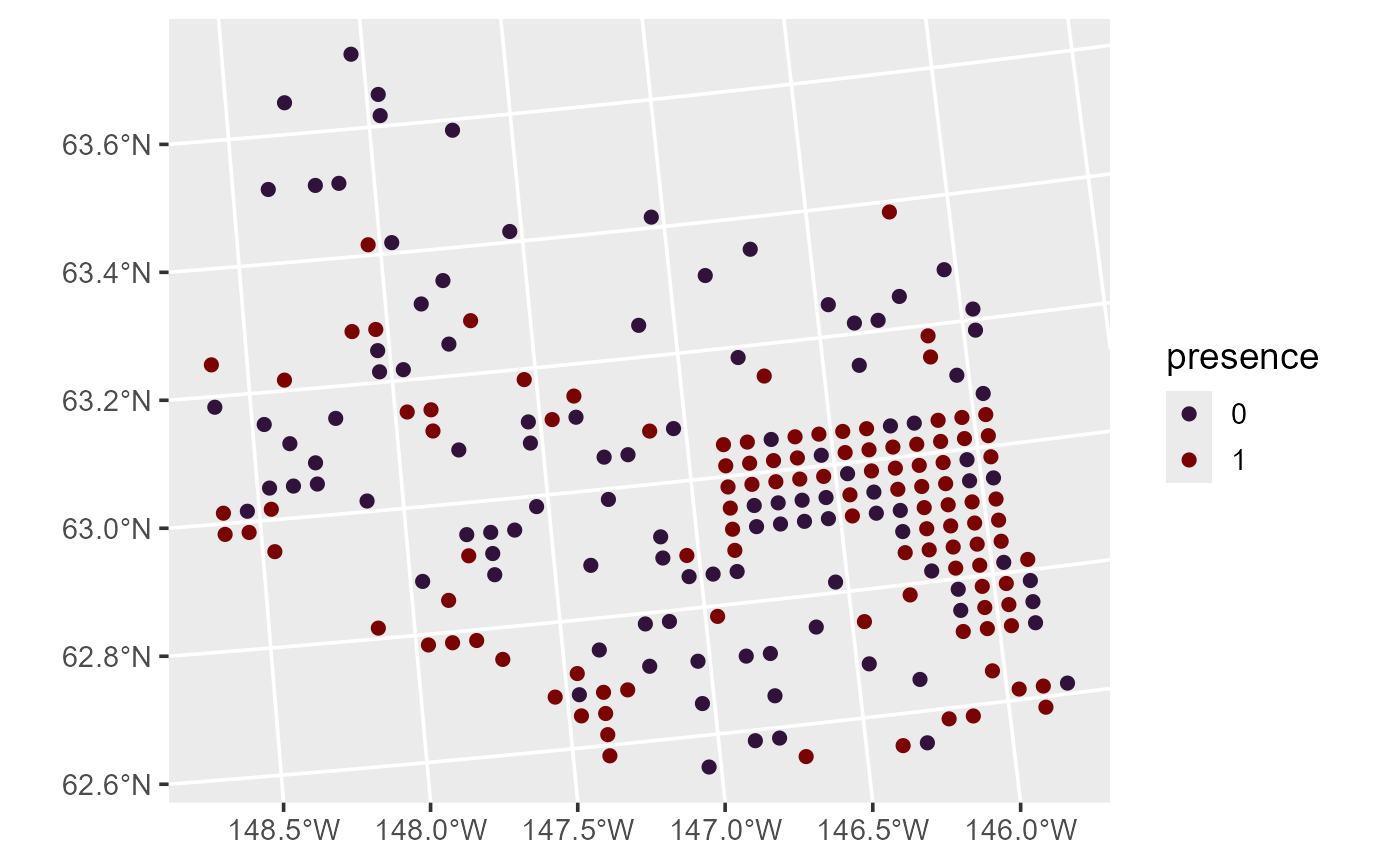

Moose presence.

There is spatial patterning in the distribution of moose presence, as moose tend to be present in the eastern and southwestern parts of the domain. This spatial pattern seems to have a directional orientation, seemingly strongest in the northwest-to-southeast direction.

Next, we visualize the elevation for each strata:

ggplot(moose, aes(color = elev)) +
  geom_sf(size = 1) + 
  facet_grid(~ strat) +
  scale_color_viridis_c()  +
  scale_y_continuous(breaks = seq(62.6, 63.6, length.out = 5)) +
  scale_x_continuous(breaks = seq(-148.5, -146, length.out = 3)) +
  theme_gray(base_size = 12)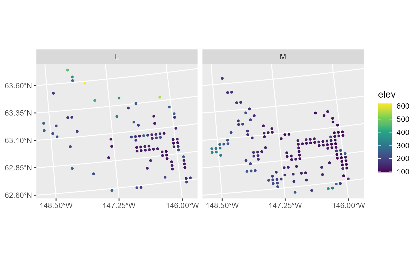

Elevation versus strata in the moose data.

There are no obvious spatial patterns in the assignment of sites to strata, while elevation is highest on the boundaries of the domain and lowest in the middle of the domain. There is spatial patterning in the distribution of moose presence, as moose tend to be present in the eastern and southwestern parts of the domain. This spatial pattern seems to have a directional orientation, seemingly strongest in the northwest-to-southeast direction.

To quantify the effects of elev, strat, and spatial dependence on moose presence, we fit three binomial (i.e., ) logistic regression models using spglm():

# model one
bin_mod <- spglm(
  formula = presence ~ elev + strat + elev:strat,
  family = "binomial",
  data = moose,
  spcov_type = "none"
)
# model two
bin_spmod <- spglm(
  formula = presence ~ elev + strat + elev:strat,
  family = "binomial",
  data = moose,
  spcov_type = "spherical"
)
# model three
bin_spmod_anis <- spglm(
  formula = presence ~ elev + strat + elev:strat,
  family = "binomial",
  data = moose,
  spcov_type = "spherical",
  anisotropy = TRUE
)

All three models have the same fixed effect structure, using elevation, strata, and their interaction to explain moose presence. The three models vary in their covariance structure. The first model, bin_mod, has no spatial covariance (\(\sigma^2_{de} = 0\)). The second model, bin_spmod has a spherical spatial covariance. The third model, bin_spmod_anis, has a spherical spatial covariance that incorporates geometric anisotropy. Geometric anisotropy allows the spatial covariance to vary with direction by evaluating the spatial covariance with \(\mathbf{H}^*\) (instead of \(\mathbf{H}\)), a matrix of distances between transformed coordinates that are rotated and scaled appropriately (Schabenberger and Gotway 2017). We evaluate the three models using AIC by running

AIC(bin_mod, bin_spmod, bin_spmod_anis)

#>                df      AIC
#> bin_mod         0 717.1627
#> bin_spmod       3 686.9031
#> bin_spmod_anis  5 677.9403

The spatial models (bin_spmod, bin_spmod_anis) have a much lower AIC than the non-spatial model (bin_mod), which suggests that the models benefit from incorporating spatial dependence. bin_spmod_anis has a lower AIC than bin_spmod, which suggests that the model benefits from incorporating directionality in the spatial dependence. Next we inspect bin_spmod_anis and later use it to predict moose presence probability at unobserved sites.

We summarize bin_spmod_anis using summary():

summary(bin_spmod_anis)

#> 
#> Call:
#> spglm(formula = presence ~ elev + strat + elev:strat, family = "binomial", 
#>     data = moose, spcov_type = "spherical", anisotropy = TRUE)
#> 
#> Deviance Residuals:
#>     Min      1Q  Median      3Q     Max 
#> -1.7970 -0.7348  0.3291  0.6855  1.7384 
#> 
#> Coefficients (fixed):
#>              Estimate Std. Error z value Pr(>|z|)   
#> (Intercept) -3.112818   1.522362  -2.045  0.04088 * 
#> elev         0.010990   0.004655   2.361  0.01824 * 
#> stratM       3.820320   1.176127   3.248  0.00116 **
#> elev:stratM -0.014020   0.006933  -2.022  0.04316 * 
#> ---
#> Signif. codes:  0 '***' 0.001 '**' 0.01 '*' 0.05 '.' 0.1 ' ' 1
#> 
#> Pseudo R-squared: 0.1119
#> 
#> Coefficients (spherical spatial covariance):
#>        de        ie     range    rotate     scale 
#> 6.580e+00 2.220e-03 1.791e+05 2.718e+00 2.154e-01 
#> attr(,"class")
#> [1] "spherical"
#> 
#> Coefficients (Dispersion for binomial family):
#> dispersion 
#>          1

The summary() output from an spglm() model is very similar to the summary() output from a base-R glm() model, returning the original function call, deviance residuals, a fixed effects coefficients table, a pseudo R-squared (which quantifies the amount of variability explained by the fixed effects), and covariance parameter coefficients. The fixed effects coefficients table provides some evidence that elevation and strata are associated with with moose presence and that the effect of elevation varies across the two strata (all \(p~\)values \(<\) 0.05).

The area under the receiver receiver operating characteristic (AUROC) curve quantifies the effectiveness of a classifier (Robin et al. 2011). It ranges from zero to one, and higher values indicate better model performance. The AUROC of bin_spmod_anis is

AUROC(bin_spmod_anis)

#> [1] 0.9403199

The plot() function returns graphics of several model diagnostics. Running

plot(bin_spmod_anis, which = c(7, 8))

Spatial dependence is a function of distance (left) and as an anisotropic level curve of equal correlation (right).

shows that the spatial dependence is evident and appears strongest in the northwest-to-southeast direction. These findings are supported by the clear spatial patterns in the data.

Recall that the tidy(), glance(), and augment() functions are particularly useful tools for manipulating and understanding fitted model objects. Thetidy()function tidies model output, returning atibble` of parameter estimates (and confidence intervals):

tidy(bin_spmod_anis, conf.int = TRUE)

#> # A tibble: 4 × 7
#>   term        estimate std.error statistic p.value conf.low conf.high
#>   <chr>          <dbl>     <dbl>     <dbl>   <dbl>    <dbl>     <dbl>
#> 1 (Intercept)  -3.11     1.52        -2.04 0.0409  -6.10    -0.129   
#> 2 elev          0.0110   0.00466      2.36 0.0182   0.00187  0.0201  
#> 3 elev:stratM  -0.0140   0.00693     -2.02 0.0432  -0.0276  -0.000431
#> 4 stratM        3.82     1.18         3.25 0.00116  1.52     6.13

By default, the fixed effects estimates are returned, but covariance parameter estimates are returned via the effects argument:

tidy(bin_spmod_anis, effects = "spcov")

#> # A tibble: 5 × 3
#>   term       estimate is_known
#>   <chr>         <dbl> <lgl>   
#> 1 de          6.58    FALSE   
#> 2 ie          0.00222 FALSE   
#> 3 range  179082.      FALSE   
#> 4 rotate      2.72    FALSE   
#> 5 scale       0.215   FALSE

The is_known column indicates whether covariance parameters were assumed known, which is possible to specify using the spcov_initial argument to spglm(). Here, all parameters were assumed unknown and then estimated.

The glance() function glances at model fit, returning a tibble of model fit statistics:

glance(bin_spmod_anis)

#> # A tibble: 1 × 10
#>       n     p  npar value   AIC  AICc   BIC logLik deviance pseudo.r.squared
#>   <int> <dbl> <int> <dbl> <dbl> <dbl> <dbl>  <dbl>    <dbl>            <dbl>
#> 1   218     4     5  668.  678.  678.  695.  -334.     161.            0.112

glances() can be used to glance at multiple models simultaneously and sorts models by ascending AICc:

glances(bin_mod, bin_spmod, bin_spmod_anis)

#> # A tibble: 3 × 11
#>   model              n     p  npar value   AIC  AICc   BIC logLik deviance
#>   <chr>          <int> <dbl> <int> <dbl> <dbl> <dbl> <dbl>  <dbl>    <dbl>
#> 1 bin_spmod_anis   218     4     5  668.  678.  678.  695.  -334.     161.
#> 2 bin_spmod        218     4     3  681.  687.  687.  697.  -340.     161.
#> 3 bin_mod          218     4     0  717.  717.  717.  717.  -359.     294.
#> # ℹ 1 more variable: pseudo.r.squared <dbl>

The augment() function augments the data with model diagnostics:

aug_mod <- augment(bin_spmod_anis)
aug_mod

#> Simple feature collection with 218 features and 8 fields
#> Geometry type: POINT
#> Dimension:     XY
#> Bounding box:  xmin: 269085 ymin: 1416151 xmax: 419057.4 ymax: 1541016
#> Projected CRS: NAD83 / Alaska Albers
#> # A tibble: 218 × 9
#>    presence  elev strat .fitted .resid    .hat   .cooksd .std.resid
#>  * <fct>    <dbl> <chr>   <dbl>  <dbl>   <dbl>     <dbl>      <dbl>
#>  1 0         469. L      -1.91  -0.527 0.0923  0.00777       -0.553
#>  2 0         362. L      -3.58  -0.235 0.00973 0.000137      -0.236
#>  3 0         173. M      -3.49  -0.246 0.00136 0.0000205     -0.246
#>  4 0         280. L      -4.41  -0.155 0.00187 0.0000113     -0.155
#>  5 0         620. L      -0.964 -0.804 0.360   0.142         -1.01 
#>  6 0         164. M      -2.64  -0.372 0.00286 0.0000996     -0.373
#>  7 0         164. M      -2.24  -0.449 0.00397 0.000202      -0.450
#>  8 0         186. L      -2.51  -0.396 0.00486 0.000192      -0.397
#>  9 0         362. L      -2.73  -0.355 0.0211  0.000692      -0.359
#> 10 0         430. L      -1.62  -0.600 0.0871  0.00941       -0.628
#> # ℹ 208 more rows
#> # ℹ 1 more variable: geometry <POINT [m]>

where .fitted are fitted values (the estimated \(f^{-1}(\mathbf{w})\), or moose presence probability), .resid are response residuals, .hat values indicate leverage, .cooksd values indicate Cook’s distance (i.e., influence), and .std.resid are standardized residuals.

The moose_preds data contains survey sites that were not sampled. We can use bin_spmod_anis to make predictions of the underlying probabilities of moose presence at these sites using predict() or augment(). predict() and augment() return the same predictions but augment() augments the prediction data with the predictions:

data("moose_preds")

spmod_anis_preds <- predict(
  bin_spmod_anis,
  newdata = moose_preds,
  type = "response",
  interval = "prediction"
)
head(spmod_anis_preds)

#>          fit         lwr       upr
#> 1 0.53625613 0.150268897 0.8831963
#> 2 0.45236331 0.106721924 0.8509940
#> 3 0.09535359 0.010375867 0.5144805
#> 4 0.10772261 0.022873507 0.3837176
#> 5 0.83772891 0.466479245 0.9682358
#> 6 0.03276524 0.003867679 0.2281264

aug_pred <- augment(
  bin_spmod_anis,
  newdata = moose_preds,
  type.predict = "response", 
  interval = "prediction"
)
aug_pred

#> Simple feature collection with 100 features and 5 fields
#> Geometry type: POINT
#> Dimension:     XY
#> Bounding box:  xmin: 269386.2 ymin: 1418453 xmax: 419976.2 ymax: 1541763
#> Projected CRS: NAD83 / Alaska Albers
#> # A tibble: 100 × 6
#>     elev strat .fitted  .lower .upper           geometry
#>  * <dbl> <chr>   <dbl>   <dbl>  <dbl>        <POINT [m]>
#>  1  143. L      0.536  0.150    0.883 (401239.6 1436192)
#>  2  324. L      0.452  0.107    0.851 (352640.6 1490695)
#>  3  158. L      0.0954 0.0104   0.514 (360954.9 1491590)
#>  4  221. M      0.108  0.0229   0.384 (291839.8 1466091)
#>  5  209. M      0.838  0.466    0.968 (310991.9 1441630)
#>  6  218. L      0.0328 0.00387  0.228 (304473.8 1512103)
#>  7  127. L      0.0381 0.00511  0.234 (339011.1 1459318)
#>  8  122. L      0.0747 0.00983  0.396 (342827.3 1463452)
#>  9  191  L      0.375  0.0410   0.893 (284453.8 1502837)
#> 10  105. L      0.142  0.0197   0.577 (391343.9 1483791)
#> # ℹ 90 more rows

Estimated moose presence probability for the moose data (obtained via fitted()) and predicted moose presence probability for the moose_preds data (obtained via predict() or augment()) are overlain below and share similar patterns:

aug_mod$type <- "mod"
aug_pred$type <- "pred"
keep_cols <- c(".fitted", "type")
aug_combined <- rbind(aug_mod[, keep_cols], aug_pred[, keep_cols])
ggplot(aug_combined, aes(color = .fitted, shape = type)) +
  geom_sf(size = 2) +
  scale_color_viridis_c(option = "H")  +
  theme_gray(base_size = 14)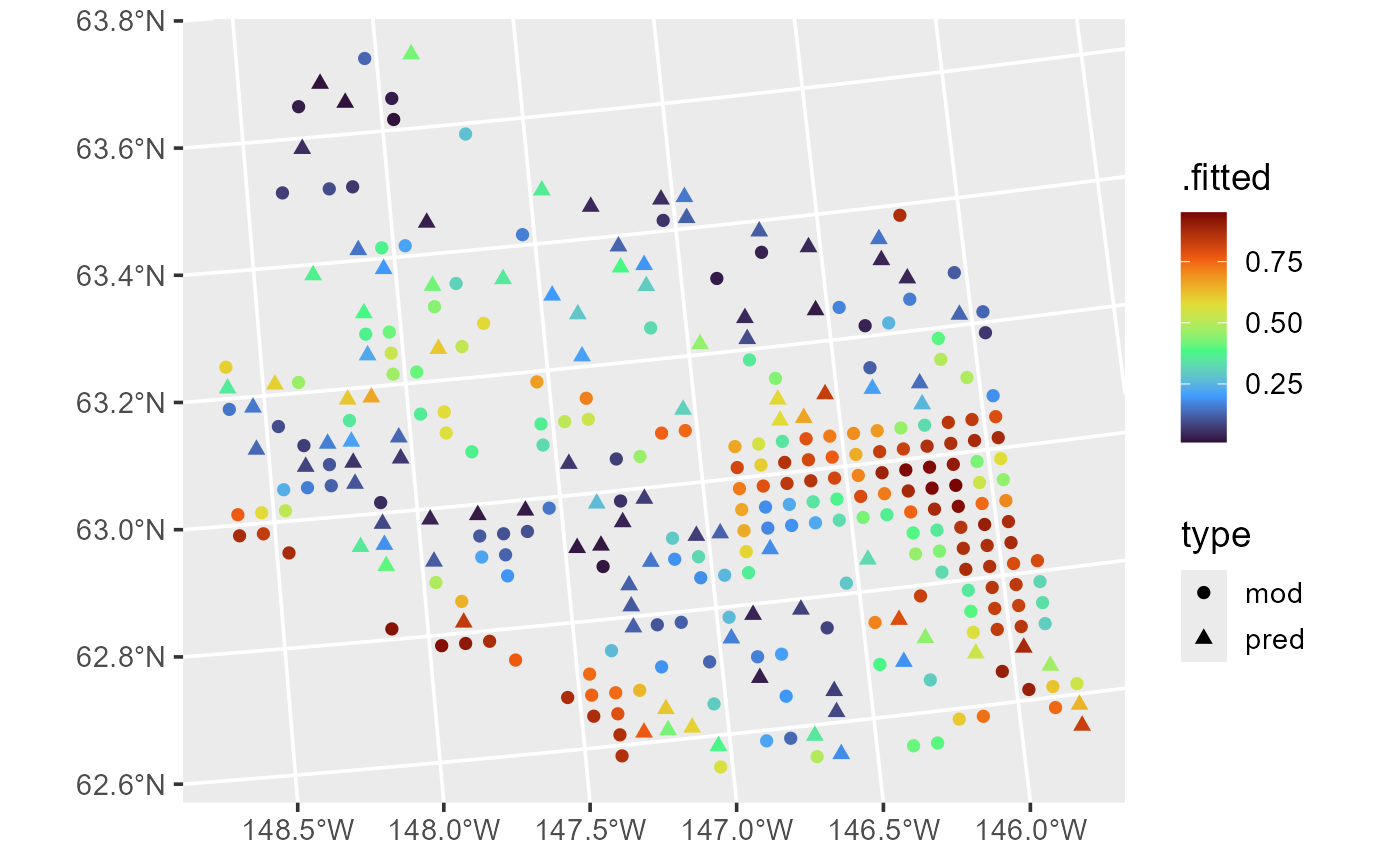

Fitted values and predictions for moose presence probability.

An application to count data

The moose data also contain the number of moose observed at each site:

ggplot(moose, aes(color = count)) +
  geom_sf(size = 2) +
  scale_color_viridis_c(option = "H")  +
  theme_gray(base_size = 14)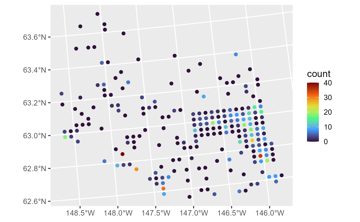

Moose counts.

The moose counts are similarly distributed as moose presence, highest in the eastern and southwestern parts of the domain. We compare two count models, Poisson and negative binomial. The Poisson model assumes the underlying process generating the counts has the same mean and variance while the negative binomial model allows for overdispersion (i.e., the variance is greater than the mean). We are interested in quantifying the effects of elev and strat on moose count, albeit using a slightly different approach than we did for moose presence. Here, we will model elevation as a fixed effect and allow this effect to change between strata, but we will model strata as a random effect to highlight additional flexibility of the spmodel package. We fit relevant Poisson and negative binomial models with a Matérn spatial covariance using spglm():

count_mod_pois <- spglm(
  count ~ elev + elev:strat,
  family = "poisson",
  data = moose,
  spcov_type = "matern",
  random = ~ (1 | strat)
)

count_mod_nb <- spglm(
  count ~ elev + elev:strat,
  family = "nbinomial",
  data = moose,
  spcov_type = "matern",
  random = ~ (1 | strat)
)

Random effects are specified in spmodel via the random argument using similar syntax as the commonly used lme4 (Bates et al. 2015) and nlme (Pinheiro and Bates 2006) R packages for non-spatial mixed models. In spmodel, ~ strat is short-hand for ~ (1 | strat). Random effects alter the covariance structure of the model, building additional correlation into the model for sites sharing a level of the random effect (here, sites within the same strata). More formally, when incorporating a random effect, the spatial generalized linear model becomes \[\begin{equation}\label{eq:spglm-rand} f(\boldsymbol{\mu}) \equiv \mathbf{w} = \mathbf{X} \boldsymbol{\beta} + \mathbf{Z}\mathbf{v} + \boldsymbol{\tau} + \boldsymbol{\epsilon}, \end{equation}\] where \(\mathbf{Z}\) is a design matrix that indexes the random effects, \(\mathbf{v}\), and \(\text{Cov}(\mathbf{v}) = \sigma^2_{v}\mathbf{I}\). Then the covariance matrix, \(\boldsymbol{\Sigma}\), becomes \(\sigma^2_v \mathbf{Z} \mathbf{Z}^\top + \sigma^2_{de}\mathbf{R} + \sigma^2_{ie}\mathbf{I}\).

Previously we compared models using AIC(), but another way to compare models is by leave-one-out cross validation (Hastie et al. 2009). In leave-one-out cross validation, each observation is held-out and the model is re-fit and used to predict the held-out observation. Then a loss statistic is computed that compares each prediction to its true value. We calculate mean-squared-prediction error (MSPE) using leave-one-out cross validation for both the Poisson and negative binomial model by running

loocv(count_mod_pois)

#> # A tibble: 1 × 3
#>    bias  MSPE RMSPE
#>   <dbl> <dbl> <dbl>
#> 1  1.37  32.0  5.66

loocv(count_mod_nb)

#> # A tibble: 1 × 3
#>    bias  MSPE RMSPE
#>   <dbl> <dbl> <dbl>
#> 1 0.291  27.1  5.20

The negative binomial model has a lower MSPE, which suggests that incorporating overdispersion improves model fit here. Tidying this fitted model we see that there is some evidence elevation is related to moose counts and that this effect changes across strata (all \(p~\)values \(< 0.1\)):

tidy(count_mod_nb)

#> # A tibble: 3 × 5
#>   term        estimate std.error statistic p.value
#>   <chr>          <dbl>     <dbl>     <dbl>   <dbl>
#> 1 (Intercept) -0.301     1.50       -0.200  0.841 
#> 2 elev         0.00590   0.00300     1.96   0.0494
#> 3 elev:stratM -0.00717   0.00408    -1.76   0.0789

The varcomp() function in spmodel apportions model variability into fixed and random components:

varcomp(count_mod_nb)

#> # A tibble: 4 × 2
#>   varcomp            proportion
#>   <chr>                   <dbl>
#> 1 Covariates (PR-sq)    0.0329 
#> 2 de                    0.498  
#> 3 ie                    0.00174
#> 4 1 | strat             0.467

Most model variability is explained by the spatially dependent random error (de) and the random effect for strata (1 | strat). Running

plot(count_mod_nb, which = c(4, 5))

Model diagnostics.

shows observations of high influence or leverage and that the standardized residuals tend to be spread out around zero.

Estimated mean moose counts for the moose data (obtained via fitted()) and predicted mean moose counts for the moose_preds data (obtained via predict() or augment()) share similar patterns and are overlain by running

aug_mod <- augment(count_mod_nb)
aug_pred <- augment(count_mod_nb, newdata = moose_preds, type.predict = "response")
aug_mod$type <- "mod"
aug_pred$type <- "pred"
keep_cols <- c(".fitted", "type")
aug_combined <- rbind(aug_mod[, keep_cols], aug_pred[, keep_cols])
ggplot(aug_combined, aes(color = .fitted, shape = type)) +
  geom_sf(size = 2) +
  scale_color_viridis_c(option = "H")  +
  theme_gray(base_size = 18)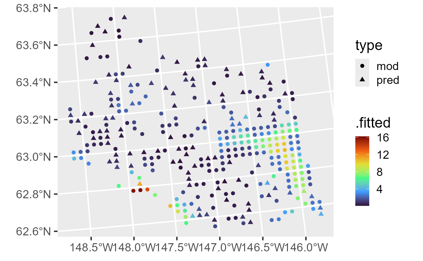

Fitted values and predictions for moose counts.

Discussion

Throughout this vignette, we have shown several features spmodel offers, including a novel application of the Laplace approximation, similarity to base R’s glm() function, over a dozen spatial covariance functions, a variety of tools available to evaluate models, inspect model diagnostics, and make predictions using ubiquitous base R functions (e.g., summary(), plot(), and predict()) and more. Spatial generalized linear models for point-referenced data (i.e., generalized geostatistical models) are fit using the spglm() function. Spatial generalized linear models for areal data (i.e., generalized spatial autoregressive models) are fit using the spgautor() function. Both functions share common structure and syntax. Spatial data are simulated in spmodel by adding an sp prefix to commonly used base R simulation functions (e.g., sprbinom()).

We appreciate feedback from users regarding spmodel. To learn more about how to provide feedback or contribute to spmodel, please visit our GitHub repository at https://github.com/USEPA/spmodel.

References

Akaike, Hirotugu. 1974. “A New Look at the Statistical Model Identification.” IEEE Transactions on Automatic Control 19 (6): 716–23.

Appelhans, Tim, Florian Detsch, Christoph Reudenbach, and Stefan Woellauer. 2022. Mapview: Interactive Viewing of Spatial Data in r. https://CRAN.R-project.org/package=mapview.

Banerjee, Sudipto, Bradley P Carlin, and Alan E Gelfand. 2014. Hierarchical Modeling and Analysis for Spatial Data. CRC press.

Bates, Douglas, Martin Mächler, Ben Bolker, and Steve Walker. 2015. “Fitting Linear Mixed-Effects Models Using lme4.” Journal of Statistical Software 67 (1): 1–48. https://doi.org/10.18637/jss.v067.i01.

Bolker, Benjamin M, Mollie E Brooks, Connie J Clark, Shane W Geange, John R Poulsen, M Henry H Stevens, and Jada-Simone S White. 2009. “Generalized Linear Mixed Models: A Practical Guide for Ecology and Evolution.” Trends in Ecology & Evolution 24 (3): 127–35.

Breslow, Norman E, and David G Clayton. 1993. “Approximate Inference in Generalized Linear Mixed Models.” Journal of the American Statistical Association 88 (421): 9–25.

Chiles, Jean-Paul, and Pierre Delfiner. 2012. Geostatistics: Modeling Spatial Uncertainty. Vol. 713. John Wiley & Sons.

Cook, R Dennis. 1979. “Influential Observations in Linear Regression.” Journal of the American Statistical Association 74 (365): 169–74.

Cressie, Noel. 1993. Statistics for Spatial Data (Revised Edition). Wiley: Hoboken, NJ. https://doi.org/10.1002/9781119115151.

Faraway, Julian J. 2016. Extending the Linear Model with R: Generalized Linear, Mixed Effects and Nonparametric Regression Models. CRC press.

Hastie, Trevor, Robert Tibshirani, Jerome H Friedman, and Jerome H Friedman. 2009. The Elements of Statistical Learning: Data Mining, Inference, and Prediction. Vol. 2. Springer.

Hoeting, Jennifer A, Richard A Davis, Andrew A Merton, and Sandra E Thompson. 2006. “Model Selection for Geostatistical Models.” Ecological Applications 16 (1): 87–98.

Lee, Youngjo, and John A Nelder. 1996. “Hierarchical Generalized Linear Models.” Journal of the Royal Statistical Society: Series B (Methodological) 58 (4): 619–56.

McCullagh, Peter, and John A. Nelder. 1989. Generalized Linear Models, Second Edition. Chapman; Hall Ltd.

Müller, Kirill, and Hadley Wickham. 2021. Tibble: Simple Data Frames. https://CRAN.R-project.org/package=tibble.

Myers, Raymond H, Douglas C Montgomery, G Geoffrey Vining, and Timothy J Robinson. 2012. Generalized Linear Models: With Applications in Engineering and the Sciences. John Wiley & Sons.

Nelder, John Ashworth, and Robert WM Wedderburn. 1972. “Generalized Linear Models.” Journal of the Royal Statistical Society: Series A (General) 135 (3): 370–84.

Pebesma, Edzer. 2018. “Simple Features for R: Standardized Support for Spatial Vector Data.” The R Journal 10 (1): 439–46. https://doi.org/10.32614/RJ-2018-009.

Pinheiro, José, and Douglas Bates. 2006. Mixed-Effects Models in s and s-PLUS. Springer science & business media.

Robin, Xavier, Natacha Turck, Alexandre Hainard, Natalia Tiberti, Frédérique Lisacek, Jean-Charles Sanchez, and Markus Müller. 2011. “pROC: An Open-Source Package for r and s+ to Analyze and Compare ROC Curves.” BMC Bioinformatics 12: 77.

Robinson, David, Alex Hayes, and Simon Couch. 2021. broom: Convert Statistical Objects into Tidy Tibbles. https://CRAN.R-project.org/package=broom.

Schabenberger, Oliver, and Carol A Gotway. 2017. Statistical Methods for Spatial Data Analysis. CRC press.

Schwarz, Gideon. 1978. “Estimating the Dimension of a Model.” The Annals of Statistics, 461–64.

Ver Hoef, Jay M, Eryn Blagg, Michael Dumelle, Philip M Dixon, Dale L Zimmerman, and Paul B Conn. 2024. “Marginal Inference for Hierarchical Generalized Linear Mixed Models with Patterned Covariance Matrices Using the Laplace Approximation.” Environmetrics, e2872.

Wickham, Hadley. 2016. ggplot2: Elegant Graphics for Data Analysis. Springer-Verlag New York. https://ggplot2.tidyverse.org.

Wood, Simon N. 2017. Generalized Additive Models: An Introduction with R. CRC press.

Michael Dumelle, Matt Higham, and Jay M. Ver Hoef