A Detailed Guide to spmodel

Introduction

spmodel is an package used to fit, summarize, and predict for a variety of spatial statistical models. The vignette provides an introduction to both the basic and advanced features of the spmodel package coupled with a brief theoretical explanation of the methods. First we give a brief theoretical introduction to spatial linear models. Then we outline the variety of methods used to estimate the parameters of spatial linear models. Then we explain how to obtain predictions at unobserved locations. Then we detail some advanced modeling features, including random effects, partition factors, anisotropy, big data approaches, and spatial generalized linear models. Finally we end with a short discussion. Before proceeding, we load spmodel by running

library(spmodel)

If using spmodel in a formal publication or report, please cite it. Citing spmodel lets us devote more resources to the package in the future. We view the spmodel citation by running

citation(package = "spmodel")

#> 
#> To cite spmodel in publications use:
#> 
#>   Dumelle M, Higham M, Ver Hoef JM (2023). spmodel: Spatial statistical
#>   modeling and prediction in R. PLOS ONE 18(3): e0282524.
#>   https://doi.org/10.1371/journal.pone.0282524
#> 
#> A BibTeX entry for LaTeX users is
#> 
#>   @Article{,
#>     title = {{spmodel}: Spatial statistical modeling and prediction in {R}},
#>     author = {Michael Dumelle and Matt Higham and Jay M. {Ver Hoef}},
#>     journal = {PLOS ONE},
#>     year = {2023},
#>     volume = {18},
#>     number = {3},
#>     pages = {1--32},
#>     doi = {10.1371/journal.pone.0282524},
#>     url = {https://doi.org/10.1371/journal.pone.0282524},
#>   }

We will create visualizations using ggplot2 (Wickham 2016), which we load by running

library(ggplot2)

ggplot2 is only installed alongside spmodel when dependencies = TRUE in install.packages(), so check that the package is installed and loaded before reproducing any of these vignette’s visualizations. We will also show code that can be used to create interactive visualizations of spatial data with mapview (Appelhans et al. 2022). mapview also has many backgrounds available that contextualize spatial data with topographical information. Before running the mapview code interactively, make sure mapview is installed and loaded.

spmodel contains various methods for generic functions defined outside of spmodel. To find relevant documentation for these methods, run help("generic.spmodel", "spmodel") (e.g., help("summary.spmodel", "spmodel"), help("predict.spmodel", "spmodel"), etc.). Note that ?generic.spmodel is shorthand for help("generic.spmodel", "spmodel"). We provide more details and examples regarding these methods and generics throughout this vignette. For a full list of spmodel functions available, see spmodel’s documentation manual.

The Spatial Linear Model

Statistical linear models are often parameterized as \[ \mathbf{y} = \mathbf{X} \boldsymbol{\beta} + \boldsymbol{\epsilon}, \] where for a sample size $n$, $\mathbf{y}$ is an $n \times 1$ column vector of response variables, $\mathbf{X}$ is an $n \times p$ design (model) matrix of explanatory variables, $\boldsymbol{\beta}$ is a $p \times 1$ column vector of fixed effects controlling the impact of $\mathbf{X}$ on $\mathbf{y}$, and $\boldsymbol{\epsilon}$ is an $n \times 1$ column vector of random errors. We typically assume that $\text{E}(\boldsymbol{\epsilon}) = \mathbf{0}$ and $\text{Cov}(\boldsymbol{\epsilon}) = \sigma^2_\epsilon \mathbf{I}$, where $\text{E}(\cdot)$ denotes expectation, $\text{Cov}(\cdot)$ denotes covariance, $\sigma^2_\epsilon$ denotes a variance parameter, and $\mathbf{I}$ denotes the identity matrix.

The model $\mathbf{y} = \mathbf{X} \boldsymbol{\beta} + \boldsymbol{\epsilon}$ assumes the elements of $\mathbf{y}$ are uncorrelated. Typically for spatial data, elements of $\mathbf{y}$ are correlated, as observations close together in space tend to be more similar than observations far apart (Tobler 1970). Failing to properly accommodate the spatial dependence in $\mathbf{y}$ can cause researchers to draw incorrect conclusions about their data. To accommodate spatial dependence in $\mathbf{y}$, an $n \times 1$ spatial random effect, $\boldsymbol{\tau}$, is added to the linear model, yielding the model \[ \mathbf{y} = \mathbf{X} \boldsymbol{\beta} + \boldsymbol{\tau} + \boldsymbol{\epsilon}, \] where $\boldsymbol{\tau}$ is independent of $\boldsymbol{\epsilon}$, $\text{E}(\boldsymbol{\tau}) = \mathbf{0}$, $\text{Cov}(\boldsymbol{\tau}) = \sigma^2_\tau \mathbf{R}$, $\mathbf{R}$ is a matrix that determines the spatial dependence structure in $\mathbf{y}$ and depends on a range parameter, $\phi$. We discuss $\mathbf{R}$ in more detail shortly. The parameter $\sigma^2_\tau$ is called the spatially dependent random error variance or partial sill. The parameter $\sigma^2_\epsilon$ is called the spatially independent random error variance or nugget. These two variance parameters are henceforth more intuitively written as $\sigma^2_{de}$ and $\sigma^2_{ie}$, respectively. The covariance of $\mathbf{y}$ is denoted $\boldsymbol{\Sigma}$ and given by $\sigma^2_{de} \mathbf{R} + \sigma^2_{ie} \mathbf{I}$. The parameters that compose this covariance are contained in the vector $\boldsymbol{\theta}$, which is called the covariance parameter vector.

The model $\mathbf{y} = \mathbf{X} \boldsymbol{\beta} + \boldsymbol{\tau} + \boldsymbol{\epsilon}$ is called the spatial linear model. The spatial linear model applies to both point-referenced and areal (i.e., lattice) data. Spatial data are point-referenced when the elements in $\mathbf{y}$ are observed at point-locations indexed by x-coordinates and y-coordinates on a spatially continuous surface with an infinite number of locations. The splm() function is used to fit spatial linear models for point-referenced data (these are sometimes called geostatistical models). One spatial covariance function available in splm() is the exponential spatial covariance function, which has an $\mathbf{R}$ matrix given by \[ \mathbf{R} = \exp(-\mathbf{M} / \phi), \] where $\mathbf{M}$ is a matrix of Euclidean distances among observations. Recall that $\phi$ is the range parameter, controlling the behavior of of the covariance function as a function of distance. Parameterizations for splm() spatial covariance types and their $\mathbf{R}$ matrices can be seen by running help("splm", "spmodel") or vignette("technical", "spmodel"). Some of these spatial covariance types (e.g., Matérn) depend on an extra parameter beyond $\sigma^2_{de}$, $\sigma^2_{ie}$, and $\phi$.

Spatial data are areal when the elements in $\mathbf{y}$ are observed as part of a finite network of polygons whose connections are indexed by a neighborhood structure. For example, the polygons may represent counties in a state that are neighbors if they share at least one boundary. Areal data are often equivalently called lattice data (Cressie 1993). The spautor() function is used to fit spatial linear models for areal data (these are sometimes called spatial autoregressive models). One spatial autoregressive covariance function available in spautor() is the simultaneous autoregressive spatial covariance function, which has an $\mathbf{R}$ matrix given by \[ \mathbf{R} = [(\mathbf{I} - \phi \mathbf{W})(\mathbf{I} - \phi \mathbf{W})^\top]^{-1}, \] where $\mathbf{W}$ is a weight matrix describing the neighborhood structure in $\mathbf{y}$. Parameterizations for spautor() spatial covariance types and their $\mathbf{R}$ matrices can be seen by running help("spautor", "spmodel") or vignette("technical", "spmodel").

One way to define $\mathbf{W}$ is through queen contiguity (Anselin, Syabri, and Kho 2010). Two observations are queen contiguous if they share a boundary. The $ij$th element of $\mathbf{W}$ is then one if observation $i$ and observation $j$ are queen contiguous and zero otherwise. Observations are not considered neighbors with themselves, so each diagonal element of $\mathbf{W}$ is zero.

Sometimes each element in the weight matrix $\mathbf{W}$ is divided by its respective row sum. This is called row-standardization. Row-standardizing $\mathbf{W}$ has several benefits, which are discussed in detail by Ver Hoef et al. (2018).

Model Fitting

In this section, we show how to use the splm() and spautor() functions to estimate parameters of the spatial linear model. We also explore diagnostic tools in spmodel that evaluate model fit. The splm() and spautor() functions share similar syntactic structure with the lm() function used to fit linear models without spatial dependence. splm() and spautor() generally require at least three arguments:

formula: a formula that describes the relationship between the response variable ($\mathbf{y}$) and explanatory variables ($\mathbf{X}$)
formula in splm() is the same as formula in lm()
data: a data.frame or sf object that contains the response variable, explanatory variables, and spatial information
spcov_type: the spatial covariance type ("exponential", "matern", "car", etc)

If data is an sf (Pebesma 2018) object, spatial information is stored in the object’s geometry. If data is a data.frame, then the x-coordinates and y-coordinates must be provided via the xcoord and ycoord arguments (for point-referenced data) or the weight matrix must be provided via the W argument (for areal data). The appendix uses the caribou data, a tibble (a special data.frame), to show how to provide spatial information via xcoord and ycoord (in splm()) or W (in spautor()).

In the following subsections, we use the point-referenced moss data, an sf object that contains data on heavy metals in mosses near a mining road in Alaska. We view the first few rows of moss by running

moss

#> Simple feature collection with 365 features and 7 fields
#> Geometry type: POINT
#> Dimension:     XY
#> Bounding box:  xmin: -445884.1 ymin: 1929616 xmax: -383656.8 ymax: 2061414
#> Projected CRS: NAD83 / Alaska Albers
#> # A tibble: 365 × 8
#>    sample field_dup lab_rep year  sideroad log_dist2road log_Zn
#>    <fct>  <fct>     <fct>   <fct> <fct>            <dbl>  <dbl>
#>  1 001PR  1         1       2001  N                 2.68   7.33
#>  2 001PR  1         2       2001  N                 2.68   7.38
#>  3 002PR  1         1       2001  N                 2.54   7.58
#>  4 003PR  1         1       2001  N                 2.97   7.63
#>  5 004PR  1         1       2001  N                 2.72   7.26
#>  6 005PR  1         1       2001  N                 2.76   7.65
#>  7 006PR  1         1       2001  S                 2.30   7.59
#>  8 007PR  1         1       2001  N                 2.78   7.16
#>  9 008PR  1         1       2001  N                 2.93   7.19
#> 10 009PR  1         1       2001  N                 2.79   8.07
#> # ℹ 355 more rows
#> # ℹ 1 more variable: geometry <POINT [m]>

We can learn more about moss by running help("moss", "spmodel"), and we can visualize the distribution of log zinc concentration in moss by running

ggplot(moss, aes(color = log_Zn)) +
  geom_sf() +
  scale_color_viridis_c() +
  theme_gray(base_size = 14)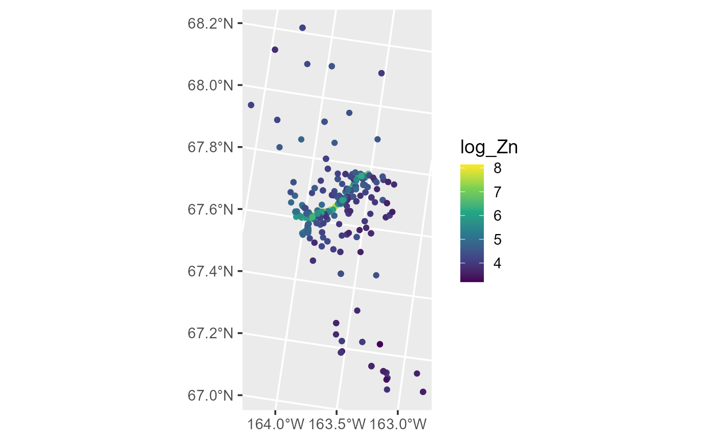

Distribution of log zinc concentration in the moss data.

Log zinc concentration can be viewed interactively in mapview by running

mapview(moss, zcol = "log_Zn")

Estimation

Generally the covariance parameters ($\boldsymbol{\theta}$) and fixed effects ($\boldsymbol{\beta}$) of the spatial linear model require estimation. The default estimation method in spmodel is restricted maximum likelihood (Patterson and Thompson 1971; Harville 1977; Wolfinger, Tobias, and Sall 1994), but the estimation method can be changed with the estmethod argument to splm() or spautor(). Maximum likelihood estimation is also available. For point-referenced data, semivariogram weighted least squares (Cressie 1985) and semivariogram composite likelihood (Curriero and Lele 1999) are additional estimation methods. The estimation method is chosen using the estmethod argument.

We estimate parameters of a spatial linear model regressing log zinc concentration (log_Zn) on log distance to a haul road (log_dist2road) using an exponential spatial covariance function by running

spmod <- splm(log_Zn ~ log_dist2road, moss, spcov_type = "exponential")

We summarize the model fit by running

summary(spmod)

#> 
#> Call:
#> splm(formula = log_Zn ~ log_dist2road, data = moss, spcov_type = "exponential")
#> 
#> Residuals:
#>     Min      1Q  Median      3Q     Max 
#> -2.6801 -1.3606 -0.8103 -0.2485  1.1298 
#> 
#> Coefficients (fixed):
#>               Estimate Std. Error z value Pr(>|z|)    
#> (Intercept)    9.76825    0.25216   38.74   <2e-16 ***
#> log_dist2road -0.56287    0.02013  -27.96   <2e-16 ***
#> ---
#> Signif. codes:  0 '***' 0.001 '**' 0.01 '*' 0.05 '.' 0.1 ' ' 1
#> 
#> Pseudo R-squared: 0.683
#> 
#> Coefficients (exponential spatial covariance):
#>        de        ie     range 
#> 3.595e-01 7.897e-02 8.237e+03

The fixed effects coefficient table contains estimates, standard errors, z-statistics, and asymptotic p-values for each fixed effect. From this table, we notice there is evidence that mean log zinc concentration significantly decreases with distance from the haul road (p-value < 2e-16). We see the fixed effect estimates by running

coef(spmod)

#>   (Intercept) log_dist2road 
#>     9.7682525    -0.5628713

The model summary also contains the exponential spatial covariance parameter estimates, which we can view by running

coef(spmod, type = "spcov")

#>           de           ie        range       rotate        scale 
#> 3.595316e-01 7.896824e-02 8.236712e+03 0.000000e+00 1.000000e+00 
#> attr(,"class")
#> [1] "exponential"

The dependent random error variance ($\sigma^2_{de}$) is estimated to be approximately 0.36 and the independent random error variance ($\sigma^2_{ie}$) is estimated to be approximately 0.079. The range ($\phi$) is estimated to be approximately 8,237. The effective range is the distance at which the spatial covariance is approximately zero. For the exponential covariance, the effective range is $3\phi$. This means that observations whose distance is greater than 24,711 meters are approximately uncorrelated. The rotate and scale parameters affect the modeling of anisotropy. By default, they are assumed to be zero and one, respectively, which means that anisotropy is not modeled (i.e., the spatial covariance is assumed isotropic, or independent of direction). We plot the fitted spatial covariance function by running

plot(spmod, which = 7)

Empirical spatial covariance of fitted model.

We can learn more about the plots available for fitted models by running help("plot.splm", "spmodel").

Model-Fit Statistics

The quality of model fit can be assessed using a variety of statistics readily available in spmodel. The first model-fit statistic we consider is the pseudo R-squared. The pseudo R-squared is a generalization of the classical R-squared from non-spatial linear models that quantifies the proportion of variability in the data explained by the fixed effects. The pseudo R-squared is defined as \[ PR2 = 1 - \frac{\mathcal{D}(\boldsymbol{\hat{\Theta}})}{\mathcal{D}(\boldsymbol{\hat{\Theta}}_0)}, \] where $\mathcal{D}(\boldsymbol{\hat{\Theta}})$ is the deviance of the fitted model indexed by parameter vector $\boldsymbol{\hat{\Theta}}$ and $\mathcal{D}(\boldsymbol{\hat{\Theta}}_0)$ is the deviance of an intercept-only model indexed by parameter vector $\boldsymbol{\hat{\Theta}}_0$. For maximum likelihood, $\hat{\boldsymbol{\Theta}} = \{\hat{\boldsymbol{\theta}}, \hat{\boldsymbol{\beta}}\}$. For restricted maximum likelihood $\hat{\boldsymbol{\Theta}} = \{\hat{\boldsymbol{\theta}}\}$.

We compute the pseudo R-squared by running We compute the pseudo R-squared by running

pseudoR2(spmod)

#> [1] 0.6829687

Roughly 68% of the variability in log zinc is explained by log distance from the road. The pseudo R-squared can be adjusted to account for the number of explanatory variables using the adjust argument. Pseudo R-squared (and the adjusted version) is most helpful for comparing models that have the same covariance structure.

The next two model-fit statistics we consider are the AIC and AICc. The AIC and AICc evaluate the fit of a model with a penalty for the number of parameters estimated. This penalty balances model fit and model parsimony. Lower AIC and AICc indicate a better balance of model fit and parsimony. The AICc is a correction to AIC for small sample sizes. As the sample size increases, AIC and AICc converge.

The spatial AIC and AICc are given by \[ \begin{split} \text{AIC} & = -2\ell(\hat{\boldsymbol{\Theta}}) + 2(|\hat{\boldsymbol{\Theta}}|) \\ \text{AICc} & = -2\ell(\hat{\boldsymbol{\Theta}}) + 2n(|\hat{\boldsymbol{\Theta}}|) / (n - |\hat{\boldsymbol{\Theta}}| - 1), \end{split} \] where $\ell(\hat{\boldsymbol{\Theta}})$ is the log-likelihood of the data evaluated at the estimated parameter vector $\hat{\boldsymbol{\Theta}}$ that maximized $\ell(\boldsymbol{\Theta})$, $|\hat{\boldsymbol{\Theta}}|$ is the dimension of $\hat{\boldsymbol{\Theta}}$, and $n$ is the sample size. As with the deviance, for maximum likelihood, $\hat{\boldsymbol{\Theta}} = \{\hat{\boldsymbol{\theta}}, \hat{\boldsymbol{\beta}}\}$, and for restricted maximum likelihood $\hat{\boldsymbol{\Theta}} = \{\hat{\boldsymbol{\theta}}\}$. There are some nuances to consider when comparing AIC across models: AIC comparisons between a model fit using restricted maximum likelihood and a model fit using maximum likelihood are meaningless, as the models are fit with different likelihoods; AIC comparisons between models fit using restricted maximum likelihood are only valid when the models have the same fixed effect structure; AIC comparisons between models fit using maximum likelihood are valid even when the models have different fixed effect structures (Pinheiro and Bates 2006).

Suppose we want to quantify the difference in model quality between the spatial model and a non-spatial model using the AIC and AICc criteria. We fit a non-spatial model in spmodel by running

lmod <- splm(log_Zn ~ log_dist2road, moss, spcov_type = "none")

This model is equivalent to one fit using lm(). We compute the spatial AIC and AICc of the spatial model and non-spatial model by running

AIC(spmod, lmod)

#>       df      AIC
#> spmod  3 373.2089
#> lmod   1 636.0635

AICc(spmod, lmod)

#>       df     AICc
#> spmod  3 373.2754
#> lmod   1 636.0745

The noticeably lower AIC and AICc of the spatial model indicate that it is a better fit to the data than the non-spatial model. Recall that these AIC and AICc comparisons are valid because both models are fit using restricted maximum likelihood (the default).

Another approach to comparing the fitted models is to perform leave-one-out cross validation (Hastie et al. 2009). In leave-one-out cross validation, a single observation is removed from the data, the model is re-fit, and a prediction is made for the held-out observation. Then, a loss metric like mean-squared-prediction error is computed and used to evaluate model fit. The lower the mean-squared-prediction error, the better the model fit. For computational efficiency, leave-one-out cross validation in spmodel is performed by first estimating $\boldsymbol{\theta}$ using all the data and then re-estimating only $\boldsymbol{\beta}$ as we predict each removed observation. We perform leave-one-out cross validation for the spatial and non-spatial model by running

loocv(spmod)

#> # A tibble: 1 × 4
#>      bias  MSPE RMSPE  cor2
#>     <dbl> <dbl> <dbl> <dbl>
#> 1 0.00655 0.111 0.333 0.886

loocv(lmod)

#> # A tibble: 1 × 4
#>       bias  MSPE RMSPE  cor2
#>      <dbl> <dbl> <dbl> <dbl>
#> 1 0.000644 0.324 0.569 0.667

The noticeably lower mean-squared-prediction error of the spatial model indicates that it is a better fit to the data than the non-spatial model.

Diagnostics

In addition to model fit metrics, spmodel provides functions that compute diagnostic metrics that help assess model assumptions and identify unusual observations.

An observation is said to have high leverage if its combination of explanatory variable values is far from the mean vector of the explanatory variables. For a non-spatial model, the leverage of the $i$th observation is the $i$th diagonal element of the hat matrix given by \[ \mathbf{H} = \mathbf{X}(\mathbf{X}^\top\mathbf{X})^{-1}\mathbf{X}^\top . \]

For a spatial model, the leverage of the $i$th observation is the $i$th diagonal element of the spatial hat matrix given by \[ \mathbf{H}^* = (\mathbf{X}^* (\mathbf{X}^{* \top} \mathbf{X})^{-1} \mathbf{X}^{* \top}) , \] where $\mathbf{X}^* = \boldsymbol{\Sigma}^{-1/2}\mathbf{X}$ and $\boldsymbol{\Sigma}^{-1/2}$ is the inverse square root of the covariance matrix, $\boldsymbol{\Sigma}$ (Montgomery, Peck, and Vining 2021). The spatial hat matrix can be viewed as the non-spatial hat matrix applied to $\mathbf{X}^*$ instead of $\mathbf{X}$. We compute the hat values (leverage) by running

hatvalues(spmod)

Larger hat values indicate more leverage, and observations with large hat values may be unusual and warrant further investigation.

The fitted value of an observation is the estimated mean response given the observation’s explanatory variable values and the model fit: \[ \hat{\mathbf{y}} = \mathbf{X} \hat{\boldsymbol{\beta}}. \] We compute the fitted values by running

fitted(spmod)

Fitted values for the spatially dependent random errors ($\boldsymbol{\tau}$), spatially independent random errors ($\boldsymbol{\epsilon}$), and random effects can also be obtained via fitted() by changing the type argument.

The residuals measure each response’s deviation from its fitted value. The response residuals are given by \[ \mathbf{e}_{r} = \mathbf{y} - \hat{\mathbf{y}}. \] We compute the response residuals of the spatial model by running

residuals(spmod)

The response residuals are typically not directly checked for linear model assumptions, as they have covariance closely resembling the covariance of $\mathbf{y}$. Pre-multiplying the residuals by $\boldsymbol{\Sigma}^{-1/2}$ yields the Pearson residuals (Myers et al. 2012): \[ \mathbf{e}_{p} = \boldsymbol{\Sigma}^{-1/2}\mathbf{e}_{r}. \] When the model is correct, the Pearson residuals have mean zero, variance approximately one, and are uncorrelated. We compute the Pearson residuals of the spatial model by running

residuals(spmod, type = "pearson")

The covariance of $\mathbf{e}_{p}$ is $(\mathbf{I} - \mathbf{H}^*)$, which is approximately $\mathbf{I}$ for large sample sizes. Explicitly dividing $\mathbf{e}_{p}$ by the respective diagonal element of $(\mathbf{I} - \mathbf{H}^*)$ yields the standardized residuals (Myers et al. 2012): \[ \mathbf{e}_{s} = \mathbf{e}_{p} \odot \frac{1}{\sqrt{(1 - \text{diag}(\mathbf{H}^*))}}, \] where $\text{diag}(\mathbf{H}^*)$ denotes the diagonal of $\mathbf{H}^*$ and $\odot$ denotes the Hadmard (element-wise) product. We compute the standardized residuals of the spatial model by running

residuals(spmod, type = "standardized")

rstandard(spmod)

When the model is correct, the standardized residuals have mean zero, variance one, and are uncorrelated. It is common to check linear model assumptions through visualizations. We can plot the standardized residuals vs fitted values by running

plot(spmod, which = 1) # figure omitted

When the model is correct, the standardized residuals should be evenly spread around zero with no discernible pattern. We can plot a normal QQ-plot of the standardized residuals by running

plot(spmod, which = 2) # figure omitted

When the standardized residuals are normally distributed, they should closely follow the normal QQ-line.

An observation is said to be influential if its omission has a large impact on model fit. Typically, this is measured using Cook’s distance (Cook and Weisberg 1982). For the non-spatial model, the Cook’s distance of the $i$th observation is denoted $\mathbf{D}$ and given by \[ \mathbf{D} = \frac{\mathbf{e}_{s}^2}{p} \odot \text{diag}(\mathbf{H}) \odot \frac{1}{(1 - \text{diag}(\mathbf{H}))}, \] where $p$ is the dimension of $\boldsymbol{\beta}$ (the number of fixed effects).

For a spatial model, the Cook’s distance of the $i$th observation is denoted $\mathbf{D}^*$ and given by \[ \mathbf{D}^* = \frac{\mathbf{e}_{s}^2}{p} \odot \text{diag}(\mathbf{H}^*) \odot \frac{1}{(1 - \text{diag}(\mathbf{H}^*))} . \] A larger Cook’s distance indicates more influence, and observations with large Cook’s distance values may be unusual and warrant further investigation. We compute Cook’s distance by running

cooks.distance(spmod)

The Cook’s distance versus leverage (hat values) can be visualized by running

plot(spmod, which = 6) # figure omitted

Though we described the model diagnostics in this subsection using $\boldsymbol{\Sigma}$, generally the covariance parameters are estimated and $\boldsymbol{\Sigma}$ is replaced with $\boldsymbol{\hat{\Sigma}}$.

The broom functions: `tidy()`, `glance()`, and `augment()`

The tidy(), glance(), and augment() functions from the broom package (Robinson, Hayes, and Couch 2021) provide convenient output for many of the model fit and diagnostic metrics discussed in the previous two sections. The tidy() function returns a tidy tibble of the coefficient table from summary():

tidy(spmod)

#> # A tibble: 2 × 5
#>   term          estimate std.error statistic p.value
#>   <chr>            <dbl>     <dbl>     <dbl>   <dbl>
#> 1 (Intercept)      9.77     0.252       38.7       0
#> 2 log_dist2road   -0.563    0.0201     -28.0       0

This tibble format makes it easy to pull out the coefficient names, estimates, standard errors, z-statistics, and p-values from the summary() output.

The glance() function returns a tidy tibble of model-fit statistics:

glance(spmod)

#> # A tibble: 1 × 9
#>       n     p  npar value   AIC  AICc logLik deviance pseudo.r.squared
#>   <int> <dbl> <int> <dbl> <dbl> <dbl>  <dbl>    <dbl>            <dbl>
#> 1   365     2     3  367.  373.  373.  -184.     363.            0.683

The glances() function is an extension of glance() that can be used to look at many models simultaneously:

glances(spmod, lmod)

#> # A tibble: 2 × 10
#>   model     n     p  npar value   AIC  AICc logLik deviance pseudo.r.squared
#>   <chr> <int> <dbl> <int> <dbl> <dbl> <dbl>  <dbl>    <dbl>            <dbl>
#> 1 spmod   365     2     3  367.  373.  373.  -184.     363.            0.683
#> 2 lmod    365     2     1  634.  636.  636.  -317.     363.            0.671

Finally, the augment() function augments the original data with model diagnostics:

augment(spmod)

#> Simple feature collection with 365 features and 7 fields
#> Geometry type: POINT
#> Dimension:     XY
#> Bounding box:  xmin: -445884.1 ymin: 1929616 xmax: -383656.8 ymax: 2061414
#> Projected CRS: NAD83 / Alaska Albers
#> # A tibble: 365 × 8
#>    log_Zn log_dist2road .fitted .resid   .hat .cooksd .std.resid
#>  *  <dbl>         <dbl>   <dbl>  <dbl>  <dbl>   <dbl>      <dbl>
#>  1   7.33          2.68    8.26 -0.928 0.0200 0.0142       1.18 
#>  2   7.38          2.68    8.26 -0.880 0.0200 0.0186       1.35 
#>  3   7.58          2.54    8.34 -0.755 0.0225 0.00482      0.647
#>  4   7.63          2.97    8.09 -0.464 0.0197 0.0305       1.74 
#>  5   7.26          2.72    8.24 -0.977 0.0215 0.131        3.45 
#>  6   7.65          2.76    8.21 -0.568 0.0284 0.0521       1.89 
#>  7   7.59          2.30    8.47 -0.886 0.0300 0.0591       1.96 
#>  8   7.16          2.78    8.20 -1.05  0.0335 0.00334      0.439
#>  9   7.19          2.93    8.12 -0.926 0.0378 0.0309       1.26 
#> 10   8.07          2.79    8.20 -0.123 0.0314 0.00847      0.723
#> # ℹ 355 more rows
#> # ℹ 1 more variable: geometry <POINT [m]>

By default, only the columns of data used to fit the model are returned alongside the diagnostics. All original columns of data are returned by setting drop to FALSE. augment() is especially powerful when the data are an sf object because model diagnostics can be easily visualized spatially. For example, we could subset the augmented object so that it only includes observations whose standardized residuals have absolute values greater than some cutoff and then visualize them spatially. To learn more about the broom functions for spatial linear models, run help("tidy.splm", "spmodel"), help("glance.splm", "spmodel"), and help("augment.splm", "spmodel").

An Areal Data Example

Next we use the seal data, an sf object that contains the log of the estimated harbor-seal trends from abundance data across polygons in Alaska, to provide an example of fitting a spatial linear model for areal data using spautor(). We view the first few rows of seal by running

seal

#> Simple feature collection with 62 features and 1 field
#> Geometry type: POLYGON
#> Dimension:     XY
#> Bounding box:  xmin: 913618.8 ymin: 1007542 xmax: 1116002 ymax: 1145054
#> Projected CRS: NAD83 / Alaska Albers
#> # A tibble: 62 × 2
#>    log_trend                                                            geometry
#>        <dbl>                                                       <POLYGON [m]>
#>  1  NA       ((1035002 1054710, 1035002 1054542, 1035002 1053542, 1035002 10525…
#>  2  -0.282   ((1037002 1039492, 1037006 1039490, 1037017 1039492, 1037035 10394…
#>  3  -0.00121 ((1070158 1030216, 1070185 1030207, 1070187 1030207, 1070211 10302…
#>  4   0.0354  ((1054906 1034826, 1054931 1034821, 1054936 1034822, 1055001 10348…
#>  5  -0.0160  ((1025142 1056940, 1025184 1056889, 1025222 1056836, 1025256 10567…
#>  6   0.0872  ((1026035 1044623, 1026037 1044605, 1026072 1044610, 1026083 10446…
#>  7  -0.266   ((1100345 1060709, 1100287 1060706, 1100228 1060706, 1100170 10607…
#>  8   0.0743  ((1030247 1029637, 1030248 1029637, 1030265 1029642, 1030328 10296…
#>  9  NA       ((1043093 1020553, 1043097 1020550, 1043101 1020550, 1043166 10205…
#> 10  -0.00961 ((1116002 1024542, 1116002 1023542, 1116002 1022542, 1116002 10215…
#> # ℹ 52 more rows

We can learn more about the data by running help("seal", "spmodel").

We can visualize the distribution of log seal trends in the seal data by running

ggplot(seal, aes(fill = log_trend)) +
  geom_sf(size = 0.75) +
  scale_fill_viridis_c() +
  theme_bw(base_size = 14)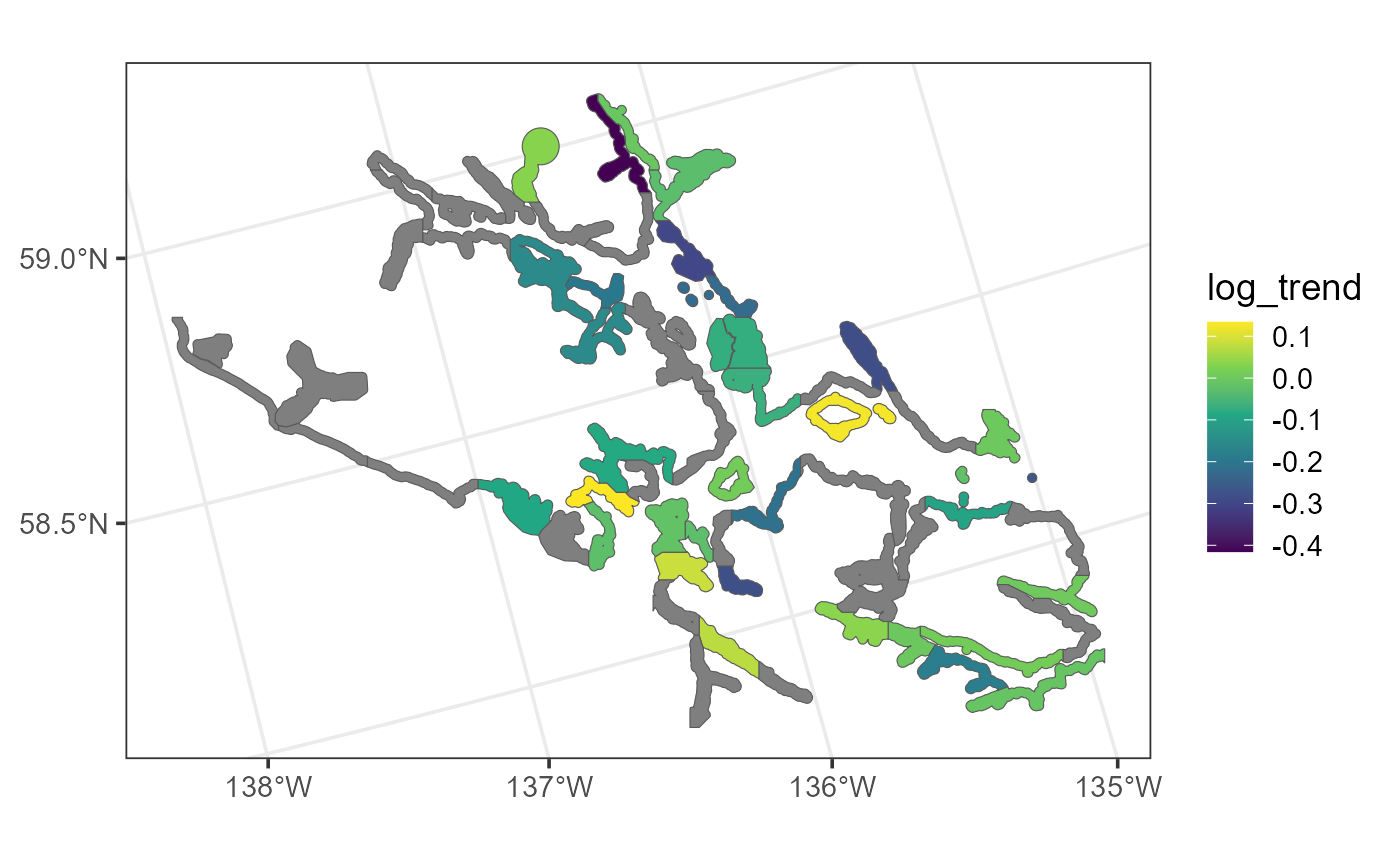

Distribution of log seal trends in the seal data. Polygons are gray if seal trends are missing.

Log trends can be viewed interactively in mapview by running

mapview(seal, zcol = "log_trend")

The gray polygons denote areas where the log trend is missing. These missing areas need to be kept in the data while fitting the model to preserve the overall neighborhood structure.

We estimate parameters of a spatial autoregressive model for log seal trends (log_trend) using an intercept-only model with a conditional autoregressive (CAR) spatial covariance by running

sealmod <- spautor(log_trend ~ 1, seal, spcov_type = "car")

If a weight matrix is not provided to spautor(), it is calculated internally using queen contiguity. Recall queen contiguity defines two observations as neighbors if they share at least one common boundary. If at least one observation has no neighbors, the extra parameter is estimated, which quantifies variability among observations without neighbors. By default, spautor() uses row standardization (Ver Hoef et al. 2018) and assumes an independent error variance (ie) of zero.

We summarize, tidy, glance at, and augment the fitted model by running

summary(sealmod)

#> 
#> Call:
#> spautor(formula = log_trend ~ 1, data = seal, spcov_type = "car")
#> 
#> Residuals:
#>      Min       1Q   Median       3Q      Max 
#> -0.34455 -0.10417  0.04410  0.07338  0.20475 
#> 
#> Coefficients (fixed):
#>             Estimate Std. Error z value Pr(>|z|)   
#> (Intercept) -0.07090    0.02497  -2.839  0.00452 **
#> ---
#> Signif. codes:  0 '***' 0.001 '**' 0.01 '*' 0.05 '.' 0.1 ' ' 1
#> 
#> Coefficients (car spatial covariance):
#>      de   range   extra 
#> 0.03252 0.42037 0.02177

tidy(sealmod)

#> # A tibble: 1 × 5
#>   term        estimate std.error statistic p.value
#>   <chr>          <dbl>     <dbl>     <dbl>   <dbl>
#> 1 (Intercept)  -0.0709    0.0250     -2.84 0.00452

glance(sealmod)

#> # A tibble: 1 × 9
#>       n     p  npar value   AIC  AICc logLik deviance pseudo.r.squared
#>   <int> <dbl> <int> <dbl> <dbl> <dbl>  <dbl>    <dbl>            <dbl>
#> 1    34     1     3 -36.9 -30.9 -30.1   18.4     33.1                0

augment(sealmod)

#> Simple feature collection with 34 features and 6 fields
#> Geometry type: POLYGON
#> Dimension:     XY
#> Bounding box:  xmin: 980001.5 ymin: 1010815 xmax: 1116002 ymax: 1145054
#> Projected CRS: NAD83 / Alaska Albers
#> # A tibble: 34 × 7
#>    log_trend .fitted  .resid   .hat .cooksd .std.resid                  geometry
#>  *     <dbl>   <dbl>   <dbl>  <dbl>   <dbl>      <dbl>             <POLYGON [m]>
#>  1  -0.282   -0.0709 -0.211  0.0161 0.0209      -1.13  ((1037002 1039492, 10370…
#>  2  -0.00121 -0.0709  0.0697 0.0473 0.0256       0.718 ((1070158 1030216, 10701…
#>  3   0.0354  -0.0709  0.106  0.0290 0.0183       0.782 ((1054906 1034826, 10549…
#>  4  -0.0160  -0.0709  0.0549 0.0228 0.00157      0.260 ((1025142 1056940, 10251…
#>  5   0.0872  -0.0709  0.158  0.0276 0.0383       1.16  ((1026035 1044623, 10260…
#>  6  -0.266   -0.0709 -0.195  0.0287 0.0530      -1.34  ((1100345 1060709, 11002…
#>  7   0.0743  -0.0709  0.145  0.0491 0.0901       1.32  ((1030247 1029637, 10302…
#>  8  -0.00961 -0.0709  0.0613 0.0122 0.00242      0.442 ((1116002 1024542, 11160…
#>  9  -0.182   -0.0709 -0.111  0.0225 0.0224      -0.986 ((1079864 1025088, 10798…
#> 10   0.00351 -0.0709  0.0744 0.0316 0.0100       0.555 ((1110363 1037056, 11103…
#> # ℹ 24 more rows

Note that for spautor() models, the ie spatial covariance parameter is assumed zero by default (and omitted from the summary() output). This default behavior can be overridden by specifying ie in the spcov_initial argument to spautor(). Also note that the pseudo R-squared is zero because there are no explanatory variables in the model (i.e., it is an intercept-only model).

Prediction

In this section, we show how to use predict() to perform spatial prediction (also called Kriging) in spmodel. We will fit a model using the point-referenced sulfate data, an sf object that contains sulfate measurements in the conterminous United States, and make predictions for each location in the point-referenced sulfate_preds data, an sf object that contains locations in the conterminous United States at which to predict sulfate.

We first visualize the distribution of the sulfate data by running

ggplot(sulfate, aes(color = sulfate)) +
  geom_sf(size = 2.5) +
  scale_color_viridis_c(limits = c(0, 45)) +
  theme_gray(base_size = 18)

We then fit a spatial linear model for sulfate using an intercept-only model with a spherical spatial covariance function by running

sulfmod <- splm(sulfate ~ 1, sulfate, spcov_type = "spherical")

Then we obtain best linear unbiased predictions (Kriging predictions) using predict(), where the newdata argument contains the locations at which to predict, storing them as a new variable in sulfate_preds called preds:

sulfate_preds$preds <- predict(sulfmod, newdata = sulfate_preds)

We can visualize the model predictions by running

ggplot(sulfate_preds, aes(color = preds)) +
  geom_sf(size = 2.5) +
  scale_color_viridis_c(limits = c(0, 45)) +
  theme_gray(base_size = 18)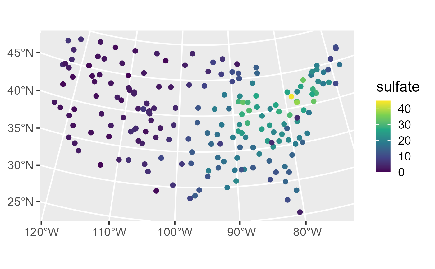

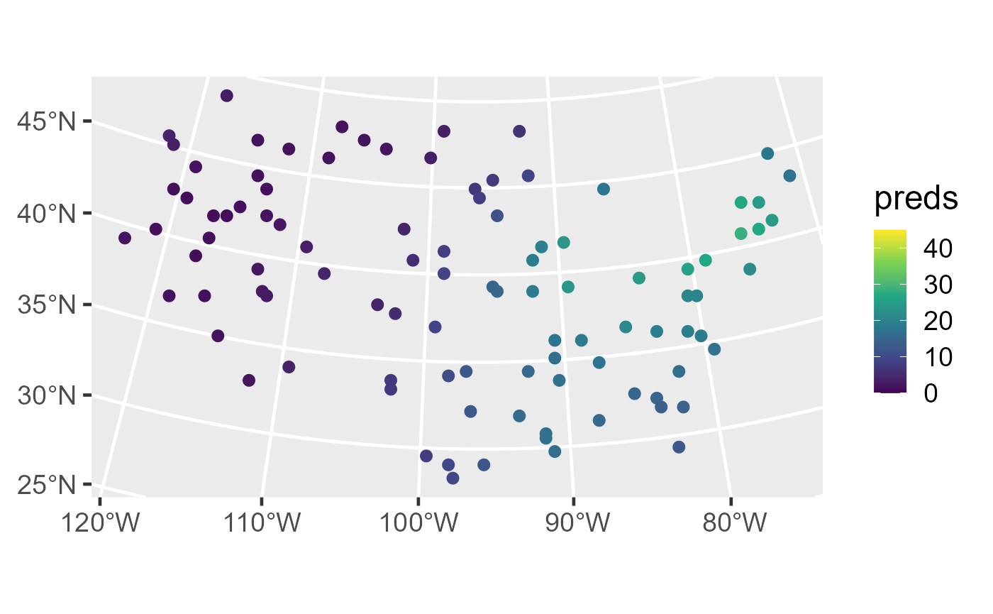
Distribution of observed sulfate (left) and sulfate predictions (right) in the conterminous United States.

Before making predictions, it is important to properly specify the newdata object. If explanatory variables were used to fit the model, the same explanatory variables must be included in newdata with the same names they have in data. Additionally, if an explanatory variable is categorical or a factor, the values of this variable in newdata must also be values in data (e.g., if a categorical variable with values "A", and "B" was used to fit the model, the corresponding variable in newdata cannot have a value "C"). If data is a data.frame, coordinates must be included in newdata with the same names as they have in data. If data is an sf object, coordinates must be included in newdata with the same geometry name as they have in data. When using projected coordinates, the projection for newdata should be the same as the projection for data.

Prediction standard errors are returned by setting the se.fit argument to TRUE:

predict(sulfmod, newdata = sulfate_preds, se.fit = TRUE)

The interval argument determines the type of interval returned. If interval is "none" (the default), no intervals are returned. If interval is "prediction", 100 * level% prediction intervals are returned (the default is 95% prediction intervals):

predict(sulfmod, newdata = sulfate_preds, interval = "prediction")

If interval is "confidence", the predictions are instead the estimated mean given each observation’s explanatory variable values. The corresponding 100 * level% confidence intervals are returned:

predict(sulfmod, newdata = sulfate_preds, interval = "confidence")

Previously we used the augment() function to augment data with model diagnostics. We can also use augment() as an alternative to predict() to augment newdata with predictions, standard errors, and intervals. We remove the model predictions from sulfate_preds before showing how augment() is used to obtain the same predictions by running

sulfate_preds$preds <- NULL

We then view the first few rows of sulfate_preds augmented with 90% prediction intervals by running

augment(sulfmod, newdata = sulfate_preds, interval = "prediction", level = 0.90)

#> Simple feature collection with 100 features and 3 fields
#> Geometry type: POINT
#> Dimension:     XY
#> Bounding box:  xmin: -2283774 ymin: 582930.5 xmax: 1985906 ymax: 3037173
#> Projected CRS: NAD83 / Conus Albers
#> # A tibble: 100 × 4
#>    .fitted .lower .upper            geometry
#>  *   <dbl>  <dbl>  <dbl>         <POINT [m]>
#>  1    1.40  -5.33   8.14  (-1771413 1752976)
#>  2   24.5   18.2   30.8    (1018112 1867127)
#>  3    8.99   2.36  15.6  (-291256.8 1553212)
#>  4   16.4    9.92  23.0    (1274293 1267835)
#>  5    4.91  -1.56  11.4  (-547437.6 1638825)
#>  6   26.7   20.4   33.0    (1445080 1981278)
#>  7    3.00  -3.65   9.66  (-1629090 3037173)
#>  8   14.3    7.97  20.6    (1302757 1039534)
#>  9    1.49  -5.08   8.06  (-1429838 2523494)
#> 10   14.4    7.97  20.8    (1131970 1096609)
#> # ℹ 90 more rows

Here, .fitted represents the predictions.

An alternative (but equivalent) approach can be used for model fitting and prediction that circumvents the need to keep data and newdata as separate objects. Suppose that observations requiring prediction are stored in data as missing (NA) values. We can add a column of missing values to sulfate_preds and then bind it together with sulfate by running

sulfate_preds$sulfate <- NA
sulfate_with_NA <- rbind(sulfate, sulfate_preds)

We can then fit a spatial linear model by running

sulfmod_with_NA <- splm(sulfate ~ 1, sulfate_with_NA, "spherical")

The missing values are ignored for model-fitting but stored in sulfmod_with_NA as newdata:

sulfmod_with_NA$newdata

#> Simple feature collection with 100 features and 1 field
#> Geometry type: POINT
#> Dimension:     XY
#> Bounding box:  xmin: -2283774 ymin: 582930.5 xmax: 1985906 ymax: 3037173
#> Projected CRS: NAD83 / Conus Albers
#> First 10 features:
#>     sulfate                  geometry
#> 198      NA  POINT (-1771413 1752976)
#> 199      NA   POINT (1018112 1867127)
#> 200      NA POINT (-291256.8 1553212)
#> 201      NA   POINT (1274293 1267835)
#> 202      NA POINT (-547437.6 1638825)
#> 203      NA   POINT (1445080 1981278)
#> 204      NA  POINT (-1629090 3037173)
#> 205      NA   POINT (1302757 1039534)
#> 206      NA  POINT (-1429838 2523494)
#> 207      NA   POINT (1131970 1096609)

We can then predict the missing values by running

predict(sulfmod_with_NA)

The call to predict() finds in sulfmod_with_NA the newdata object and is equivalent to

predict(sulfmod_with_NA, newdata = sulfmod_with_NA$newdata)

We can also use augment() to make the predictions on the data set with missing values by running

augment(sulfmod_with_NA, newdata = sulfmod_with_NA$newdata)

#> Simple feature collection with 100 features and 2 fields
#> Geometry type: POINT
#> Dimension:     XY
#> Bounding box:  xmin: -2283774 ymin: 582930.5 xmax: 1985906 ymax: 3037173
#> Projected CRS: NAD83 / Conus Albers
#> # A tibble: 100 × 3
#>    sulfate .fitted            geometry
#>  *   <dbl>   <dbl>         <POINT [m]>
#>  1      NA    1.40  (-1771413 1752976)
#>  2      NA   24.5    (1018112 1867127)
#>  3      NA    8.99 (-291256.8 1553212)
#>  4      NA   16.4    (1274293 1267835)
#>  5      NA    4.91 (-547437.6 1638825)
#>  6      NA   26.7    (1445080 1981278)
#>  7      NA    3.00  (-1629090 3037173)
#>  8      NA   14.3    (1302757 1039534)
#>  9      NA    1.49  (-1429838 2523494)
#> 10      NA   14.4    (1131970 1096609)
#> # ℹ 90 more rows

Unlike predict(), augment() explicitly requires the newdata argument be specified in order to obtain predictions. Omitting newdata (e.g., running augment(sulfmod_with_NA)) returns model diagnostics, not predictions.

For areal data models fit with spautor(), predictions cannot be computed at locations that were not incorporated in the neighborhood structure used to fit the model. Thus, predictions are only possible for observations in data whose response values are missing (NA), as their locations are incorporated into the neighborhood structure. For example, we make predictions of log seal trends at the missing polygons by running

predict(sealmod)

We can also use augment() to make the predictions:

augment(sealmod, newdata = sealmod$newdata)

#> Simple feature collection with 28 features and 2 fields
#> Geometry type: POLYGON
#> Dimension:     XY
#> Bounding box:  xmin: 913618.8 ymin: 1007542 xmax: 1115097 ymax: 1132682
#> Projected CRS: NAD83 / Alaska Albers
#> # A tibble: 28 × 3
#>    log_trend  .fitted                                                   geometry
#>  *     <dbl>    <dbl>                                              <POLYGON [m]>
#>  1        NA -0.115   ((1035002 1054710, 1035002 1054542, 1035002 1053542, 1035…
#>  2        NA -0.00908 ((1043093 1020553, 1043097 1020550, 1043101 1020550, 1043…
#>  3        NA -0.0602  ((1099737 1054310, 1099752 1054262, 1099788 1054278, 1099…
#>  4        NA -0.0359  ((1099002 1036542, 1099134 1036462, 1099139 1036431, 1099…
#>  5        NA -0.0723  ((1076902 1053189, 1076912 1053179, 1076931 1053179, 1076…
#>  6        NA -0.0548  ((1070501 1046969, 1070317 1046598, 1070308 1046542, 1070…
#>  7        NA -0.0976  ((1072995 1054942, 1072996 1054910, 1072997 1054878, 1072…
#>  8        NA -0.0714  ((960001.5 1127667, 960110.8 1127542, 960144.1 1127495, 9…
#>  9        NA -0.0825  ((1031308 1079817, 1031293 1079754, 1031289 1079741, 1031…
#> 10        NA -0.0592  ((998923.7 1053647, 998922.5 1053609, 998950 1053631, 999…
#> # ℹ 18 more rows

Advanced Features

spmodel offers several advanced features for fitting spatial linear models. We briefly discuss some of these features next using the moss data, the moose data, and some simulated data. Technical details for each advanced feature can be seen by running vignette("technical", "spmodel").

Fixing Spatial Covariance Parameters

We may desire to fix specific spatial covariance parameters at a particular value. Perhaps some parameter value is known, for example. Or perhaps we want to compare nested models where a reduced model uses a fixed parameter value while the full model estimates the parameter. Fixing spatial covariance parameters while fitting a model is possible using the spcov_initial argument to splm() and spautor(). The spcov_initial argument takes an spcov_initial object (run help("spcov_initial", "spmodel") for more). spcov_initial objects can also be used to specify initial values used during optimization, even if they are not assumed to be fixed. By default, spmodel uses a grid search to find suitable initial values to use during optimization.

As an example, suppose our goal is to compare a model with an exponential covariance with dependent error variance, independent error variance, and range parameters to a model that assumes the independent random error variance parameter (nugget) is zero. First, the spcov_initial object is specified for the latter model:

init <- spcov_initial("exponential", ie = 0, known = "ie")
print(init)

#> $initial
#> ie 
#>  0 
#> 
#> $is_known
#>   ie 
#> TRUE 
#> 
#> attr(,"class")
#> [1] "exponential"

The init output shows that the ie parameter has an initial value of zero that is assumed to be known. Next the model is fit:

spmod_red <- splm(log_Zn ~ log_dist2road, moss, spcov_initial = init)

Notice that because the spcov_initial object contains information about the spatial covariance type, the spcov_type argument is not required when spcov_initial is provided. We can use glances() to glance at both models:

glances(spmod, spmod_red)

#> # A tibble: 2 × 10
#>   model         n     p  npar value   AIC  AICc logLik deviance pseudo.r.squared
#>   <chr>     <int> <dbl> <int> <dbl> <dbl> <dbl>  <dbl>    <dbl>            <dbl>
#> 1 spmod       365     2     3  367.  373.  373.  -184.     363.            0.683
#> 2 spmod_red   365     2     2  378.  382.  382.  -189.     374.            0.703

The lower AIC and AICc of the full model compared to the reduced model indicates that the independent random error variance is important to the model. A likelihood ratio test comparing the full and reduced models is also possible using anova().

Another application of fixing spatial covariance parameters involves calculating their profile likelihood confidence intervals (Box and Cox 1964). Before calculating a profile likelihood confidence interval for $\boldsymbol{\Theta}_i$, the $i$th element of a general parameter vector $\boldsymbol{\Theta}$, it is necessary to obtain $-2\ell(\hat{\boldsymbol{\Theta}})$, minus twice the log-likelihood evaluated at the estimated parameter vector, $\hat{\boldsymbol{\Theta}}$. Then a $(1 - \alpha)$% profile likelihood confidence interval is the set of values for $\boldsymbol{\Theta}_i$ such that $2\ell(\hat{\boldsymbol{\Theta}}) - 2\ell(\hat{\boldsymbol{\Theta}}_{-i}) \leq \chi^2_{1, 1 - \alpha}$, where $\ell(\hat{\boldsymbol{\Theta}}_{-i})$ is the value of the log-likelihood maximized after fixing $\boldsymbol{\Theta}_i$ and optimizing over the remaining parameters, $\boldsymbol{\Theta}_{-i}$, and $\chi^2_{1, 1 - \alpha}$ is the $1 - \alpha$ quantile of a chi-squared distribution with one degree of freedom. The result follows from inverting a likelihood ratio test comparing the full model to a reduced model that fixes the value of $\boldsymbol{\Theta}_i$. Because this approach requires refitting the model many times for different fixed values of $\boldsymbol{\Theta}_i$, it can be computationally intensive. This approached can be generalized to yield joint profile likelihood confidence intervals cases when $i$ has dimension greater than one.

Fitting and Predicting for Multiple Models

Fitting multiple models is possible with a single call to splm() or spautor() when spcov_type is a vector with length greater than one or spcov_initial is a list (with length greater than one) of spcov_initial objects. We fit three separate spatial linear models using the exponential spatial covariance, spherical spatial covariance, and no spatial covariance by running

spmods <- splm(sulfate ~ 1, sulfate, spcov_type = c("exponential", "spherical", "none"))

spmods is list whose names indicate the spatial covariance type and whose values indicate the model fit for that spatial covariance type. Generic functions can be called individually for each list element. For example, we can augment the the model fit using the exponential covariance function with diagnostics by running

augment(spmods$exponential)

#> Simple feature collection with 197 features and 6 fields
#> Geometry type: POINT
#> Dimension:     XY
#> Bounding box:  xmin: -2292550 ymin: 386181.1 xmax: 2173345 ymax: 3090370
#> Projected CRS: NAD83 / Conus Albers
#> # A tibble: 197 × 7
#>    sulfate .fitted .resid    .hat   .cooksd .std.resid           geometry
#>  *   <dbl>   <dbl>  <dbl>   <dbl>     <dbl>      <dbl>        <POINT [m]>
#>  1  12.9      5.92   7.00 0.00334 0.00161      -0.694  (817738.8 1080571)
#>  2  20.2      5.92  14.2  0.00256 0.00192       0.865  (914593.6 1295545)
#>  3  16.8      5.92  10.9  0.00259 0.000395      0.390  (359574.1 1178228)
#>  4  16.2      5.92  10.3  0.00239 0.000363      0.390  (265331.9 1239089)
#>  5   7.86     5.92   1.93 0.00202 0.00871      -2.07   (304528.8 1453636)
#>  6  15.4      5.92   9.43 0.00201 0.000240      0.345  (162932.8 1451625)
#>  7   0.986    5.92  -4.94 0.00380 0.000966     -0.503  (-1437776 1568022)
#>  8   0.425    5.92  -5.50 0.0138  0.00584      -0.646  (-1572878 1125529)
#>  9   3.58     5.92  -2.34 0.00673 0.0000148    -0.0467 (-1282009 1204889)
#> 10   2.38     5.92  -3.54 0.0123  0.0000139    -0.0335 (-1972775 1464991)
#> # ℹ 187 more rows

Or we can find the AIC of the model fit using the spherical covariance function by running

AIC(spmods$spherical)

#> [1] 1143.202

The glances() and predict() functions can work directly with spmods, calling glances() and predict() on each list element and then organizing the results. We glance at each fitted model object by running

glances(spmods)

#> # A tibble: 3 × 10
#>   model         n     p  npar value   AIC  AICc logLik deviance pseudo.r.squared
#>   <chr>     <int> <dbl> <int> <dbl> <dbl> <dbl>  <dbl>    <dbl>            <dbl>
#> 1 spherical   197     1     3 1137. 1143. 1143.  -569.     196.                0
#> 2 exponent…   197     1     3 1140. 1146. 1146.  -570.     196.                0
#> 3 none        197     1     1 1448. 1450. 1450.  -724.     196                 0

We predict newdata separately for each fitted model object by running

predict(spmods, newdata = sulfate_preds)

Random Effects

Non-spatial random effects incorporate additional sources of variability into model fitting. They are accommodated in spmodel using similar syntax as for random effects in the nlme (Pinheiro and Bates 2006) and lme4 (Bates et al. 2015) packages. Random effects are specified via a formula passed to the random argument. Next we show two examples that incorporate random effects into the spatial linear model using the moss data.

The first example explores random intercepts for the sample variable. The sample variable indexes each unique location, which can have replicate observations due to field duplicates (field_dup) and lab replicates (lab_rep). There are 365 observations in moss at 318 unique locations, which means that 47 observations in moss are either field duplicates or lab replicates. It is likely that the repeated observations at a location are correlated with one another. We can incorporate this repeated-observation correlation by creating a random intercept for each level of sample. We model the random intercepts for sample by running

rand1 <- splm(
  log_Zn ~ log_dist2road,
  moss,
  spcov_type = "exponential",
  random = ~ sample
)

Note that ~ sample is shorthand for (1 | sample), which is more explicit notation that indicates random intercepts for each level of sample.

The second example adds a random intercept for year, which creates extra correlation for observations within a year. It also adds a random slope for log_dist2road within year, which lets the effect of log_dist2road vary between years. We fit this model by running

rand2 <- splm(
  log_Zn ~ log_dist2road,
  moss,
  spcov_type = "exponential",
  random = ~ sample + (log_dist2road | year)
)

Note that sample + (log_dist2road | year) is shorthand for (1 | sample) + (log_dist2road | year). If only random slopes within a year are desired (and no random intercepts), a - 1 is given to the relevant portion of the formula: (log_dist2road - 1 | year). When there is more than one term in random, each term must be surrounded by parentheses (recall that the random intercept shorthand automatically includes relevant parentheses). More examples of random effect syntax are provided in the appendix.

We compare the AIC of the models by running

glances(rand1, rand2)

#> # A tibble: 2 × 10
#>   model     n     p  npar value   AIC  AICc logLik deviance pseudo.r.squared
#>   <chr> <int> <dbl> <int> <dbl> <dbl> <dbl>  <dbl>    <dbl>            <dbl>
#> 1 rand2   365     2     6  190.  202.  202.  -94.9     363.            0.215
#> 2 rand1   365     2     4  335.  343.  343. -168.      363.            0.661

The rand2 model has the lowest AIC.

It is possible to fix random effect variances using the randcov_initial argument, and randcov_initial can also be used to set initial values for optimization.

Partition Factors

A partition factor is a variable that allows observations to be uncorrelated when they are from different levels of the partition factor. Partition factors are specified in spmodel by providing a formula with a single variable to the partition_factor argument. Suppose that for the moss data, we want observations in different years (year) to be uncorrelated. We fit a model that treats year as a partition factor by running

part <- splm(
  log_Zn ~ log_dist2road,
  moss,
  spcov_type = "exponential",
  partition_factor = ~ year
)

Anisotropy

An isotroptic spatial covariance function (for point-referenced data) behaves similarly in all directions (i.e., is independent of direction) as a function of distance. An anisotropic covariance function does not behave similarly in all directions as a function of distance. Consider the spatial covariance imposed by an eastward-moving wind pattern. A one-unit distance in the x-direction likely means something different than a one-unit distance in the y-direction. Below are ellipses for an isotropic and anisotropic covariance function centered at the origin (a distance of zero).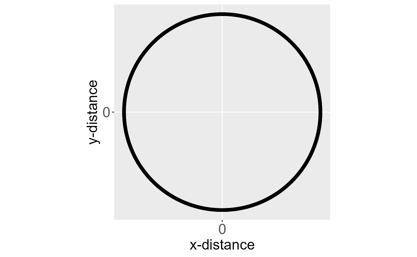

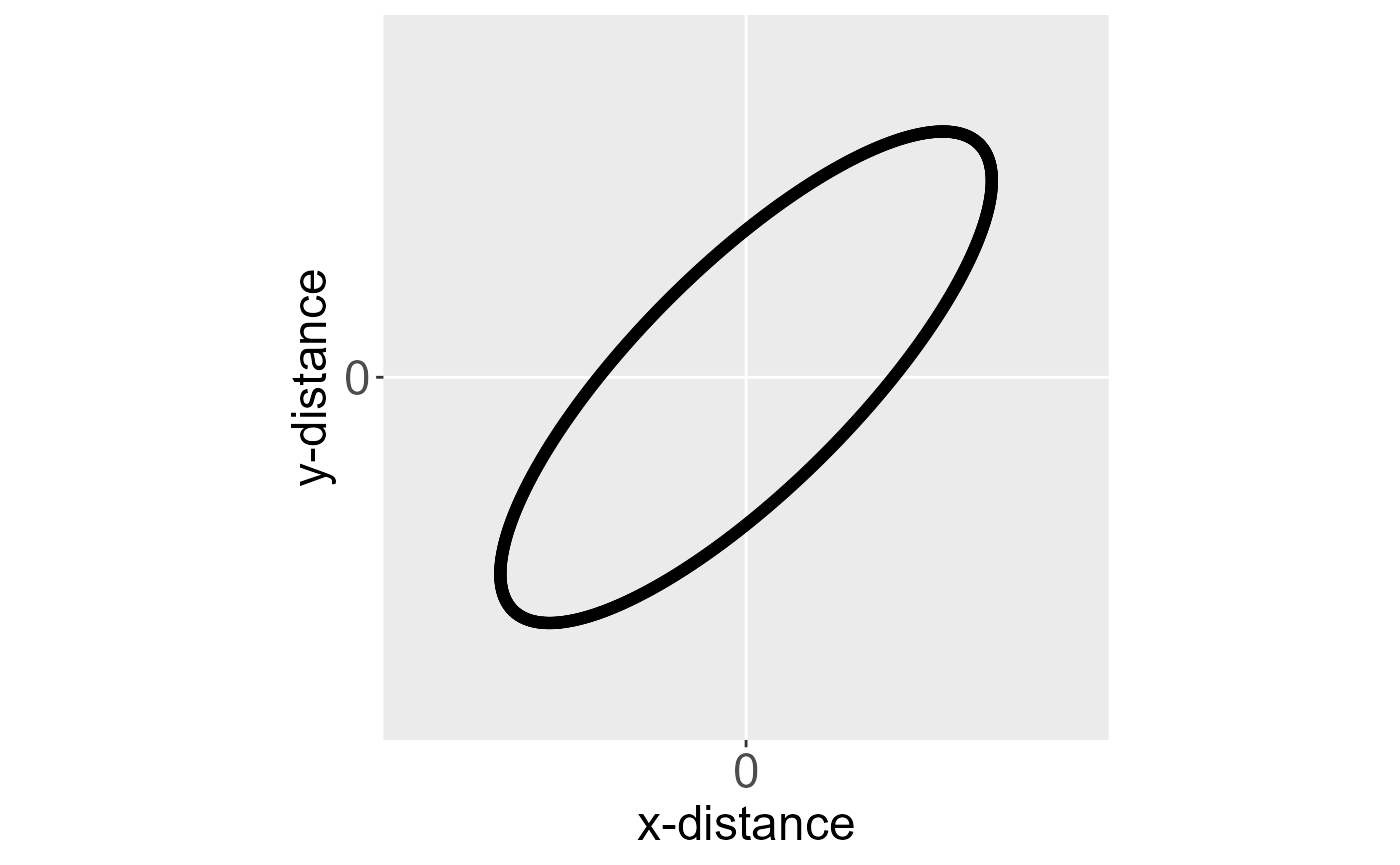
Ellipses for an isotropic (left) and anisotropic (right) covariance function centered at the origin. The black outline of each ellipse is a level curve of equal correlation.

The black outline of each ellipse is a level curve of equal correlation. The left ellipse (a circle) represents an isotropic covariance function. The distance at which the correlation between two observations lays on the level curve is the same in all directions. The right ellipse represents an anisotropic covariance function. The distance at which the correlation between two observations lays on the level curve is different in different directions.

Accounting for anisotropy involves a rotation and scaling of the x-coordinates and y-coordinates such that the spatial covariance function that uses these transformed distances is isotropic. We use the anisotropy argument to splm() to fit a model with anisotropy by running

spmod_anis <- splm(
  log_Zn ~ log_dist2road,
  moss,
  spcov_type = "exponential",
  anisotropy = TRUE
)
summary(spmod_anis)

#> 
#> Call:
#> splm(formula = log_Zn ~ log_dist2road, data = moss, spcov_type = "exponential", 
#>     anisotropy = TRUE)
#> 
#> Residuals:
#>     Min      1Q  Median      3Q     Max 
#> -2.5279 -1.2239 -0.7202 -0.1921  1.1659 
#> 
#> Coefficients (fixed):
#>               Estimate Std. Error z value Pr(>|z|)    
#> (Intercept)    9.54798    0.22291   42.83   <2e-16 ***
#> log_dist2road -0.54601    0.01855  -29.44   <2e-16 ***
#> ---
#> Signif. codes:  0 '***' 0.001 '**' 0.01 '*' 0.05 '.' 0.1 ' ' 1
#> 
#> Pseudo R-squared: 0.7048
#> 
#> Coefficients (exponential spatial covariance):
#>        de        ie     range    rotate     scale 
#> 3.561e-01 6.812e-02 8.732e+03 2.435e+00 4.753e-01 
#> attr(,"class")
#> [1] "exponential"

The rotate parameter is between zero and $\pi$ radians and represents the angle of a clockwise rotation of the ellipse such that the major axis of the ellipse is the new x-axis and the minor axis of the ellipse is the new y-axis. The scale parameter is between zero and one and represents the ratio of the distance between the origin and the edge of the ellipse along the minor axis to the distance between the origin and the edge of the ellipse along the major axis. Below shows a transformation that turns an anisotropic ellipse into an isotropic one (i.e., a circle). This transformation requires rotating the coordinates clockwise by rotate and then scaling them the reciprocal of scale. The transformed coordinates are then used instead of the original coordinates to compute distances and spatial covariances.

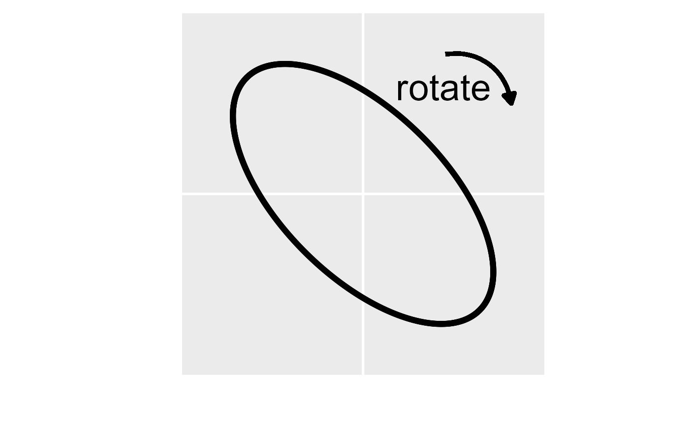
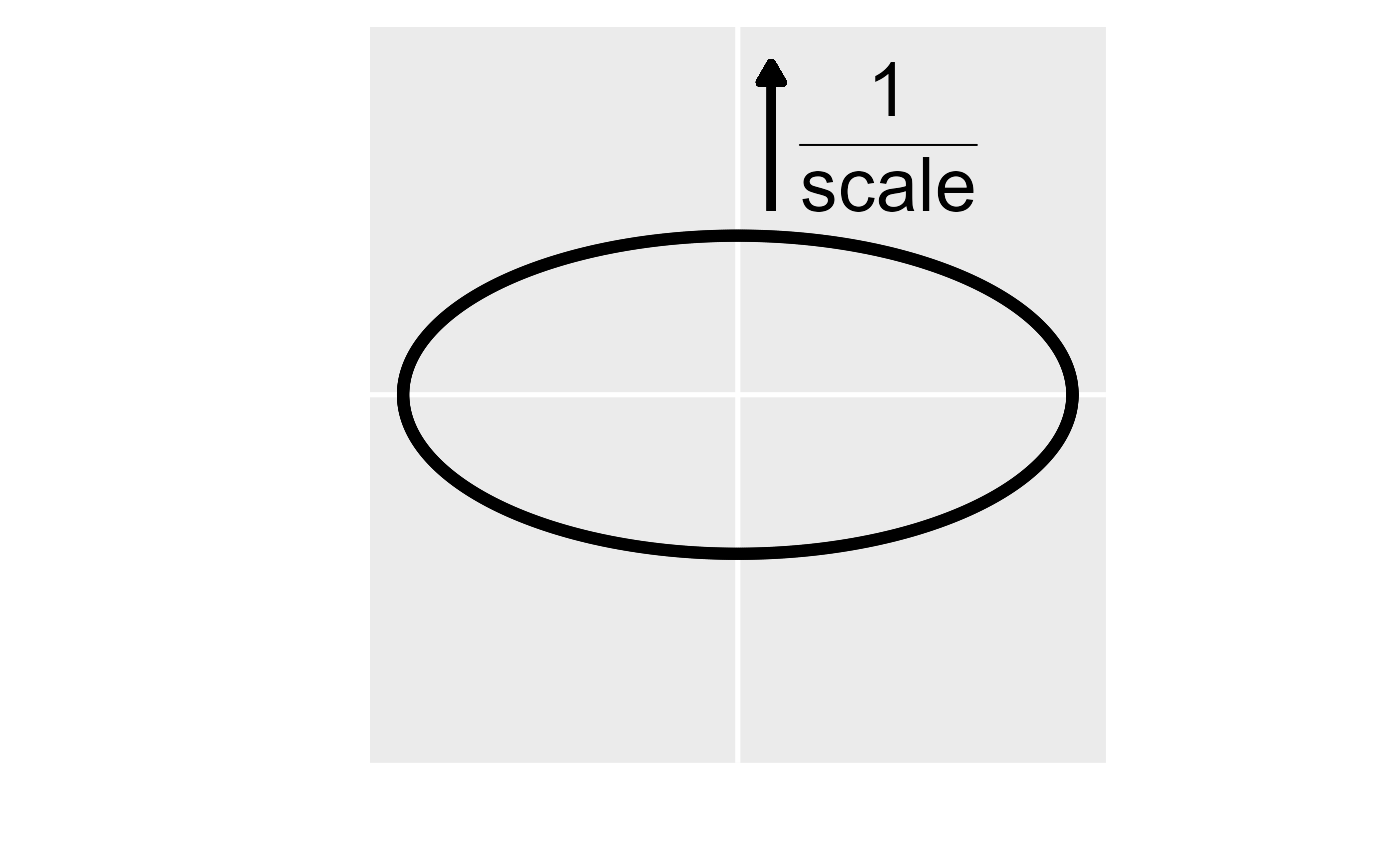
$A visual representation of the anisotropy transformation. In the left figure, the first step is to rotate the anisotropic ellipse clockwise by the \texttt{rotate} parameter (here \texttt{rotate} is 0.75$\pi$ radians or 135 degrees). In the middle figure, the second step is to scale the y axis by the reciprocal of the \texttt{scale} parameter (here \texttt{scale} is 0.5). In the right figure, the anisotropic ellipse has been transformed into an isotropic one (i.e., a circle). The transformed coordinates are then used instead of the original coordinates to compute distances and spatial covariances.$ $A visual representation of the anisotropy transformation. In the left figure, the first step is to rotate the anisotropic ellipse clockwise by the \texttt{rotate} parameter (here \texttt{rotate} is 0.75$\pi$ radians or 135 degrees). In the middle figure, the second step is to scale the y axis by the reciprocal of the \texttt{scale} parameter (here \texttt{scale} is 0.5). In the right figure, the anisotropic ellipse has been transformed into an isotropic one (i.e., a circle). The transformed coordinates are then used instead of the original coordinates to compute distances and spatial covariances.$ $A visual representation of the anisotropy transformation. In the left figure, the first step is to rotate the anisotropic ellipse clockwise by the \texttt{rotate} parameter (here \texttt{rotate} is 0.75$\pi$ radians or 135 degrees). In the middle figure, the second step is to scale the y axis by the reciprocal of the \texttt{scale} parameter (here \texttt{scale} is 0.5). In the right figure, the anisotropic ellipse has been transformed into an isotropic one (i.e., a circle). The transformed coordinates are then used instead of the original coordinates to compute distances and spatial covariances.$

A visual representation of the anisotropy transformation. In the left figure, the first step is to rotate the anisotropic ellipse clockwise by the parameter (here is 0.75$\pi$ radians or 135 degrees). In the middle figure, the second step is to scale the y axis by the reciprocal of the parameter (here is 0.5). In the right figure, the anisotropic ellipse has been transformed into an isotropic one (i.e., a circle). The transformed coordinates are then used instead of the original coordinates to compute distances and spatial covariances.

Note that specifying an initial value for rotate that is different from zero, specifying an initial value for scale that is different from one, or assuming either rotate or scale are unknown in spcov_initial will cause splm() to fit a model with anisotropy (and will override anisotropy = FALSE). Estimating anisotropy parameters is only possible for maximum likelihood and restricted maximum likelihood estimation, but fixed anisotropy parameters can be accommodated for semivariogram weighted least squares or semivariogram composite likelihood estimation. Also note that anisotropy is not relevant for areal data because the spatial covariance function depends on a neighborhood structure instead of distances between points.

Simulating Spatial Data

The sprnorm() function is used to simulate normal (Gaussian) spatial data. To use sprnorm(), the spcov_params() function is used to create an spcov_params object. The spcov_params() function requires the spatial covariance type and parameter values. We create an spcov_params object by running

sim_params <- spcov_params("exponential", de = 5, ie = 1, range = 0.5)

We set a reproducible seed and then simulate data at 3000 random locations in the unit square using the spatial covariance parameters in sim_params by running

set.seed(0)
n <- 3000
x <- runif(n)
y <- runif(n)
sim_coords <- tibble::tibble(x, y)
sim_response <- sprnorm(sim_params, data = sim_coords, xcoord = x, ycoord = y)
sim_data <- tibble::tibble(sim_coords, sim_response)

We can visualize the simulated data by running

ggplot(sim_data, aes(x = x, y = y, color = sim_response)) +
  geom_point(size = 1.5) +
  scale_color_viridis_c(limits = c(-7, 7)) + 
  theme_gray(base_size = 18)

There is noticeable spatial patterning in the response variable (sim_response). The default mean in sprnorm() is zero for all observations, though a mean vector can be provided using the mean argument. The default number of samples generated in sprnorm() is one, though this can be changed using the samples argument. Because sim_data is a tibble (data.frame) and not an sf object, the columns in sim_data representing the x-coordinates and y-coordinates must be provided to sprnorm().

Note that the output from coef(object, type = "spcov") is a spcov_params object. This is useful if we want to simulate data given the estimated spatial covariance parameters from a fitted model. Random effects are incorporated into simulation via the randcov_params argument.

Big Data

The computational cost associated with model fitting is exponential in the sample size for all estimation methods. For maximum likelihood and restricted maximum likelihood, the computational cost of estimating $\boldsymbol{\theta}$ is cubic. For semivariogram weighted least squares and semivariogram composite likelihood, the computational cost of estimating $\boldsymbol{\theta}$ is quadratic. The computational cost associated with estimating $\boldsymbol{\beta}$ and prediction is cubic, regardless of estimation method. Typically, samples sizes approaching 10,000 make the computational cost of model fitting and prediction infeasible, which necessitates the use of big data methods. spmodel offers big data methods for model fitting of point-referenced data via the local argument to splm(). The method is capable of quickly fitting models with hundreds of thousands of observations. Because of the neighborhood structure of areal data, the big data methods used for point-referenced data do not apply to areal data. Thus, there is no big data method for areal data or local argument to spautor(), so model fitting sample sizes cannot be too large

spmodel offers big data methods for prediction of point-referenced data or areal data via the local argument to predict(). This method is capable of quickly predicting hundreds of thousands of observations. To show how to use spmodel for big data estimation and prediction, we use the sim_data data from the previous section. Because sim_data is a tibble (data.frame) and not an sf object, the columns in data representing the x-coordinates and y-coordinates must be explicitly provided to splm().

Next we briefly discuss model fitting and prediction for big data in spmodel, but further details are provided by Ver Hoef, Dumelle, et al. (2023).

Model Fitting

spmodel uses a “local spatial indexing” (SPIN) approach for big data model fitting of point-referenced data. Observations are first assigned an index. Then for the purposes of model fitting, observations with different indexes are assumed uncorrelated. Assuming observations with different indexes are uncorrelated induces sparsity in the covariance matrix, which greatly reduces the computational time of operations that involve the covariance matrix.

The local argument to splm() controls the big data options. local is a list with several arguments. The arguments to the local list control the method used to assign the indexes, the number of observations with the same index, the number of unique indexes, variance adjustments to the covariance matrix of $\hat{\boldsymbol{\beta}}$, whether or not to use parallel processing, and if parallel processing is used, the number of cores.

Big data are most simply accommodated by setting local to TRUE. This is shorthand for

local = list(method = "kmeans", size = 100, var_adjust = "theoretical", parallel = FALSE),

which assigns observations to index groups based on k-means clustering (MacQueen 1967), ensures each index group has approximately 100 observations, uses the theoretically-correct variance adjustment, and does not use parallel processing.

local1 <- splm(sim_response ~ 1, sim_data, spcov_type = "exponential", 
               xcoord = x, ycoord = y, local = TRUE)
summary(local1)

#> 
#> Call:
#> splm(formula = sim_response ~ 1, data = sim_data, spcov_type = "exponential", 
#>     xcoord = x, ycoord = y, local = TRUE)
#> 
#> Residuals:
#>     Min      1Q  Median      3Q     Max 
#> -4.9414 -1.2573 -0.0527  1.3783  6.6322 
#> 
#> Coefficients (fixed):
#>             Estimate Std. Error z value Pr(>|z|)  
#> (Intercept)  -1.1149     0.6416  -1.738   0.0823 .
#> ---
#> Signif. codes:  0 '***' 0.001 '**' 0.01 '*' 0.05 '.' 0.1 ' ' 1
#> 
#> Coefficients (exponential spatial covariance):
#>     de     ie  range 
#> 2.3112 1.0260 0.2395

Instead of using local = TRUE, we can explicitly set local. For example, we can fit a model using random assignment with 60 groups, use the pooled variance adjustment, and use parallel processing with two cores by running

local2_list <- list(method = "random", groups = 60, var_adjust = "pooled",
                    parallel = TRUE, ncores = 2)
local2 <- splm(sim_response ~ 1, sim_data, spcov_type = "exponential", 
               xcoord = x, ycoord = y, local = local2_list)

Likelihood-based statistics like AIC(), AICc(), logLik(), and deviance() should not be used to compare a model fit with a big data approximation to a model fit without a big data approximation.

Prediction

For point-referenced data, spmodel uses a “local neighborhood” approach for big data prediction. Each prediction is computed using a subset of the observed data instead of all of the observed data. Before further discussing big data prediction, we simulate 1000 locations in the unit square requiring prediction:

n_pred <- 1000
x <- runif(n_pred)
y <- runif(n_pred)
sim_preds <- tibble::tibble(x = x, y = y)

The local argument to predict() controls the big data options. local is a list with several arguments. The arguments to the local list control the method used to subset the observed data, the number of observations in each subset, whether or not to use parallel processing, and if parallel processing is used, the number of cores.

The simplest way to accommodate big data prediction is to set local to TRUE. This is shorthand for local = list(method = "covariance", size = 100, parallel = FALSE), which implies that, for each location requiring prediction, only the 100 observations in the data most correlated with it are used in the computation and parallel processing is not used. Using the local1 fitted model, we store these predictions as a variable called preds in the sim_preds data by running

sim_preds$preds <- predict(local1, newdata = sim_preds, local = TRUE)

The predictions are visualized by running

ggplot(sim_preds, aes(x = x, y = y, color = preds)) +
  geom_point(size = 1.5) +
  scale_color_viridis_c(limits = c(-7, 7)) + 
  theme_gray(base_size = 18)

They display a similar pattern as the observed data.

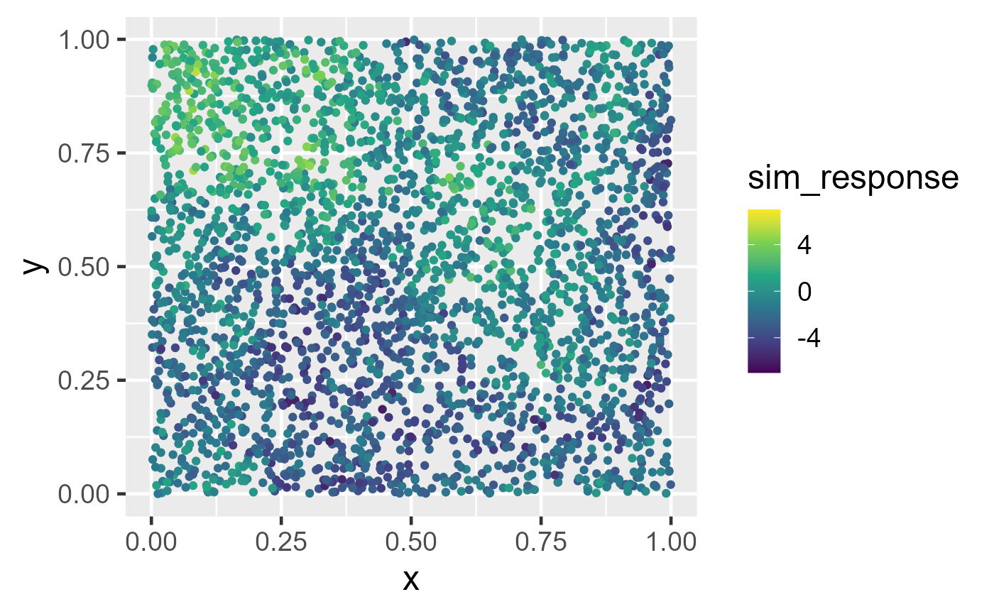
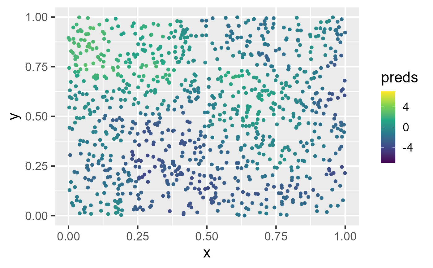
Observed data and big data predictions at unobserved locations. In the left figure, spatial data are simulated in the unit square. A spatial linear model is fit using the default big data approximation for model-fitting. In the right figure, predictions are made using the fitted model and the default big data approximation for prediction.

Instead of using local = TRUE, we can explicitly set local:

pred_list <- list(method = "distance", size = 30, parallel = TRUE, ncores = 2)
predict(local1, newdata = sim_preds, local = pred_list)

This code implies that uniquely for each location requiring prediction, only the 30 observations in the data closest to it (in terms of Euclidean distance) are used in the computation and parallel processing is used with two cores.

For areal data, no local neighborhood approximation exists because of the data’s underlying neighborhood structure. Thus, all of the data must be used to compute predictions, and by consequence, method and size are not components of the local list. The only components of the local list for areal data are parallel and ncores.

Random Forest Spatial Residual Models

Random forest spatial residual models are used for prediction. They combine aspects of random forest prediction and spatial linear model prediction, which can lead to significant improvements in predictive accuracy compared to standard random forest prediction (Fox, Ver Hoef, and Olsen 2020). To fit a random forest spatial residual model, use splmRF() (for point-referenced data) or spautorRF() (for areal data). These functions require at least one explanatory variable be specified, so we add an explanatory variable called var to sulfate and sulfate_preds for illustrative purposes.

sulfate$var <- rnorm(NROW(sulfate))
sulfate_preds$var <- rnorm(NROW(sulfate_preds))

Then we fit a random forest spatial residual model by running

sprfmod <- splmRF(sulfate ~ var, sulfate, spcov_type = "exponential")

And we make predictions by running

predict(sprfmod, newdata = sulfate_preds)

Spatial Generalized Linear Models

When building spatial linear models, the response vector $\mathbf{y}$ is typically assumed Gaussian (given $\mathbf{X}$). Relaxing this assumption on the distribution of $\mathbf{y}$ yields a rich class of spatial generalized linear models that can describe binary data, proportion data, count data, and skewed data that is parameterized as \[ g(\boldsymbol{\mu}) = \boldsymbol{\eta} = \mathbf{X} \boldsymbol{\beta} + \boldsymbol{\tau} + \boldsymbol{\epsilon}, \] where $g(\cdot)$ is called a link function, $\boldsymbol{\mu}$ is the mean of $\mathbf{y}$, and the remaining terms $\mathbf{X}$, $\boldsymbol{\beta}$, $\boldsymbol{\tau}$, $\boldsymbol{\epsilon}$ represent the same quantities as for the spatial linear models. The link function, $g(\cdot)$, “links” a function of $\boldsymbol{\mu}$ to the linear term $\boldsymbol{\eta}$ , denoted here as $\mathbf{X} \boldsymbol{\beta} + \boldsymbol{\tau} + \boldsymbol{\epsilon}$, which is familiar from spatial linear models. Note that the linking of $\boldsymbol{\mu}$ to $\boldsymbol{\eta}$ applies element-wise to each vector. Each link function $g(\cdot)$ has a corresponding inverse link function, $g^{-1}(\cdot)$. The inverse link function “links” a function of $\boldsymbol{\eta}$ to $\boldsymbol{\mu}$. Notice that for spatial generalized linear models, we are not modeling $\mathbf{y}$ directly as we do for spatial linear models, but rather we are modeling a function of the mean of $\mathbf{y}$. Also notice that $\boldsymbol{\eta}$ is unconstrained but $\boldsymbol{\mu}$ is usually constrained in some way (e.g., positive).

The model $g(\boldsymbol{\mu}) = \boldsymbol{\eta} = \mathbf{X} \boldsymbol{\beta} + \boldsymbol{\tau} + \boldsymbol{\epsilon}$ is called the spatial generalized linear model. spmodel allows fitting of spatial generalized linear models when $\mathbf{y}$ is a binomial (or Bernoulli), beta, Poisson, negative binomial, gamma, or inverse Gaussian random vector via the Laplace approximation and restricted maximum likelihood estimation or maximum likelihood estimation – Ver Hoef, Blagg, et al. (2023) provide further details. For binomial and beta $\mathbf{y}$, the logit link function is defined as $g(\boldsymbol{\mu}) = \ln(\frac{\boldsymbol{\mu}}{1 - \boldsymbol{\mu}}) = \boldsymbol{\eta}$, and the inverse logit link function is defined as $g^{-1}(\boldsymbol{\eta}) = \frac{\exp(\boldsymbol{\eta})}{1 + \exp(\boldsymbol{\eta})} = \boldsymbol{\mu}$. For Poisson, negative binomial, gamma, and inverse Gaussian $\mathbf{y}$, the log link function is defined as $g(\boldsymbol{\mu}) = \ln(\boldsymbol{\mu}) = \boldsymbol{\eta}$, and the inverse log link function is defined as $g^{-1}(\boldsymbol{\eta}) = \exp(\boldsymbol{\eta}) = \boldsymbol{\mu}$. Full parameterizations of these distributions are given in the technical details vignette, which can be viewed by running vignette("technical", "spmodel").

All advanced features available in spmodel for spatial linear models are also available for spatial generalized linear models. This means that spatial generalized linear models in spmodel can accommodate fixing spatial covariance parameters, fitting and predicting for multiple models, random effects (on the link scale), partition factors, anisotropy (on the link scale), simulation, big data, and prediction.

Model Fitting

As with spatial linear models, spatial generalized linear models are fit in spmodel for point-referenced and areal data. The spglm() function is used to fit spatial generalized linear models for point-referenced data, and the spgautor() function is used to fit spatial generalized linear models for areal data. spglm() and spgautor() share similar syntax with splm() and spautor(), respectively, though one additional argument is required:

family: the generalized linear model family (i.e., the distribution of $\mathbf{y}$). family can be binomial, beta, poisson, nbinomial, Gamma, or inverse.gaussian.
family uses similar syntax as the family argument in glm().
One difference between family in spglm() compared to family in glm() is that the link function is fixed in spglm().

As with splm() and spautor(), the data argument to spglm() and spgautor() can be an sf object or data.frame (with appropriate coordinate or weight matrix information). Additionally, all arguments to splm() and spautor() are also available for spglm() and spgautor().

Next we show the basic features and syntax of spglm() using the moose data. We study the impact of elevation (elev) on the presence of moose (presence) observed at a site location in Alaska. presence equals one if at least one moose was observed at the site and zero otherwise. We view the first few rows of the moose data by running

moose

#> Simple feature collection with 218 features and 4 fields
#> Geometry type: POINT
#> Dimension:     XY
#> Bounding box:  xmin: 269085 ymin: 1416151 xmax: 419976.2 ymax: 1541763
#> Projected CRS: NAD83 / Alaska Albers
#> First 10 features:
#>        elev strat count presence                 geometry
#> 1  468.9167     L     0        0 POINT (293542.6 1541016)
#> 2  362.3125     L     0        0 POINT (298313.1 1533972)
#> 3  172.7500     M     0        0 POINT (281896.4 1532516)
#> 4  279.6250     L     0        0 POINT (298651.3 1530264)
#> 5  619.6000     L     0        0 POINT (311325.3 1527705)
#> 6  164.1250     M     0        0 POINT (291421.5 1518398)
#> 7  163.5000     M     0        0 POINT (287298.3 1518035)
#> 8  186.3500     L     0        0 POINT (279050.9 1517324)
#> 9  362.3125     L     0        0 POINT (346145.9 1512479)
#> 10 430.5000     L     0        0 POINT (321354.6 1509966)

We can visualize the distribution of moose presence (presence) by running

ggplot(moose, aes(color = presence)) +
  geom_sf(size = 2) +
  scale_color_viridis_d(option = "H") +
  theme_gray(base_size = 14)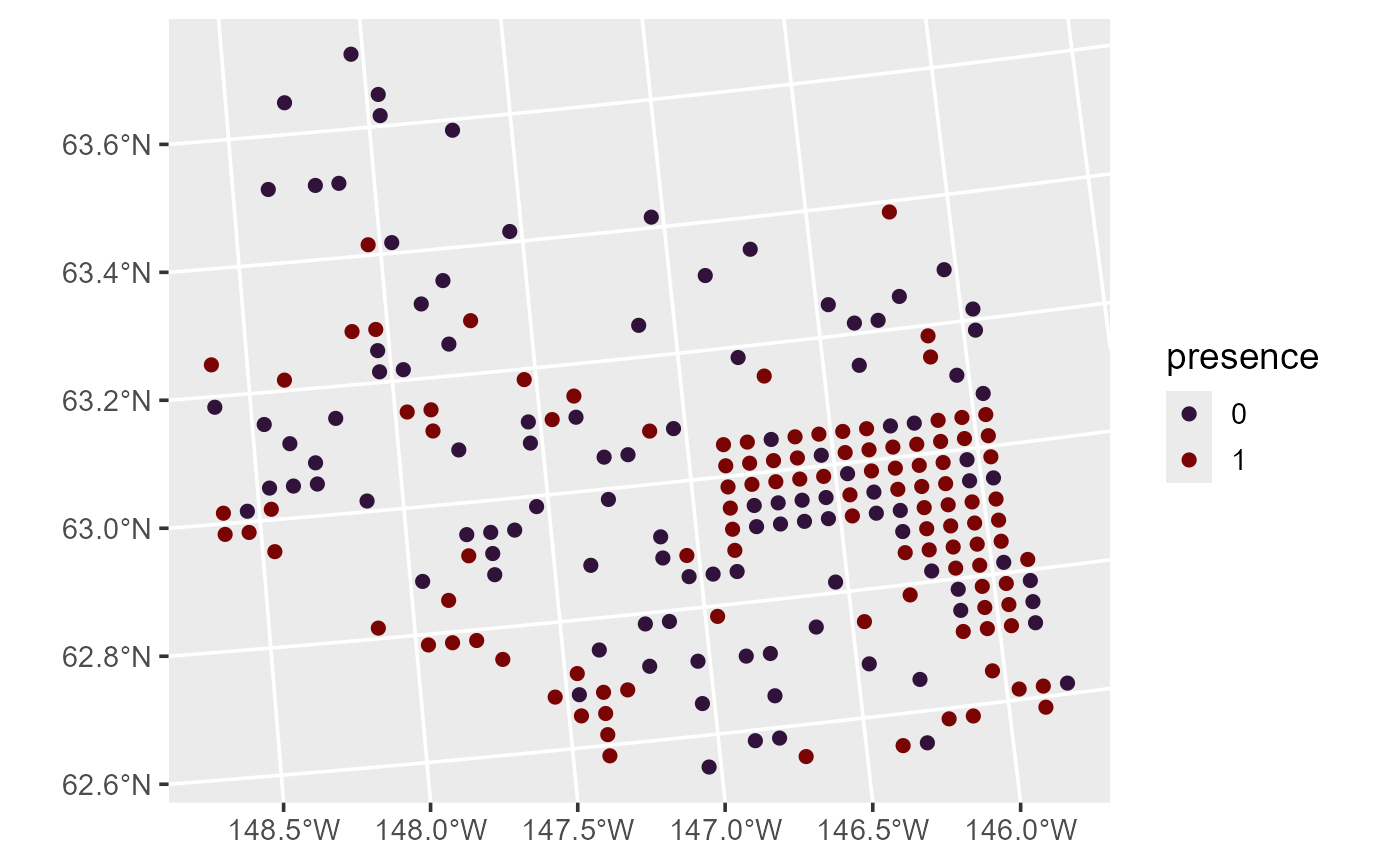

Distribution of moose presence in Alaska. presence equals one if at least one moose was observed at the site and zero otherwise.

One example of a generalized linear model is a binomial (e.g., logistic) regression model. Binomial regression models are often used to model presence data such as these. To quantify the relationship between moose presence and elevation, we fit a spatial binomial regression model (a specific spatial generalized linear model) by running

binmod <- spglm(presence ~ elev, family = "binomial",
                data  = moose, spcov_type = "exponential")

The estimation method is specified via the estmethod argument, which has a default value of "reml" for restricted maximum likelihood. The other estimation method is "ml" for maximum likelihood.

We summarize the fitted model by running

summary(binmod)

#> 
#> Call:
#> spglm(formula = presence ~ elev, family = "binomial", data = moose, 
#>     spcov_type = "exponential")
#> 
#> Deviance Residuals:
#>     Min      1Q  Median      3Q     Max 
#> -1.5249 -0.8114  0.5600  0.8306  1.5757 
#> 
#> Coefficients (fixed):
#>              Estimate Std. Error z value Pr(>|z|)
#> (Intercept) -0.874038   1.140953  -0.766    0.444
#> elev         0.002365   0.003184   0.743    0.458
#> 
#> Pseudo R-squared: 0.00311
#> 
#> Coefficients (exponential spatial covariance):
#>        de        ie     range 
#> 3.746e+00 4.392e-03 3.203e+04 
#> 
#> Coefficients (Dispersion for binomial family):
#> dispersion 
#>          1

Similar to summaries of glm() objects, summaries of spglm() objects include the original function call, summary statistics of the deviance residuals, and a coefficients table of fixed effects. The logit of moose presence probability does not appear to be related to elevation, as evidenced by the large p-value associated with the asymptotic z-test. A pseudo r-squared is also returned, which quantifies the proportion of variability explained by the fixed effects. The spatial covariance parameters and dispersion parameter are also returned. The dispersion parameter is estimated in some spatial generalized linear models and changes the mean-variance relationship of $\mathbf{y}$. For binomial regression models, the dispersion parameter is not estimated and is always fixed at one.

We tidy, glance, and augment the fitted model by running

tidy(binmod)

#> # A tibble: 2 × 5
#>   term        estimate std.error statistic p.value
#>   <chr>          <dbl>     <dbl>     <dbl>   <dbl>
#> 1 (Intercept) -0.874     1.14       -0.766   0.444
#> 2 elev         0.00237   0.00318     0.743   0.458

glance(binmod)

#> # A tibble: 1 × 9
#>       n     p  npar value   AIC  AICc logLik deviance pseudo.r.squared
#>   <int> <dbl> <int> <dbl> <dbl> <dbl>  <dbl>    <dbl>            <dbl>
#> 1   218     2     3  692.  698.  698.  -346.     190.          0.00311

augment(binmod)

#> Simple feature collection with 218 features and 7 fields
#> Geometry type: POINT
#> Dimension:     XY
#> Bounding box:  xmin: 269085 ymin: 1416151 xmax: 419057.4 ymax: 1541016
#> Projected CRS: NAD83 / Alaska Albers
#> # A tibble: 218 × 8
#>    presence  elev .fitted .resid    .hat  .cooksd .std.resid
#>  * <fct>    <dbl>   <dbl>  <dbl>   <dbl>    <dbl>      <dbl>
#>  1 0         469.  0.150  -0.571 0.0500  0.00904      -0.586
#>  2 0         362.  0.107  -0.477 0.0168  0.00198      -0.481
#>  3 0         173.  0.104  -0.468 0.00213 0.000235     -0.469
#>  4 0         280.  0.0939 -0.444 0.00616 0.000615     -0.445
#>  5 0         620.  0.198  -0.664 0.136   0.0402       -0.714
#>  6 0         164.  0.130  -0.528 0.00260 0.000364     -0.528
#>  7 0         164.  0.135  -0.538 0.00269 0.000392     -0.539
#>  8 0         186.  0.166  -0.603 0.00332 0.000607     -0.604
#>  9 0         362.  0.168  -0.606 0.0245  0.00474      -0.614
#> 10 0         430.  0.225  -0.714 0.0528  0.0150       -0.734
#> # ℹ 208 more rows
#> # ℹ 1 more variable: geometry <POINT [m]>

Prediction

For spatial generalized linear models, we are predicting the mean of the process generating the observation (which includes the spatial effects) rather than the observation itself. We make predictions of moose presence probability at the locations in moose_preds by running

moose_preds$preds <- predict(binmod, newdata = moose_preds, type = "response")

The type argument specifies whether predictions are returned on the link or response (inverse link) scale.

We visualize these predictions by running

ggplot(moose_preds, aes(color = preds)) + 
  geom_sf(size = 2) +
  scale_color_viridis_c(limits = c(0, 1), option = "H") + 
  theme_gray(base_size = 14)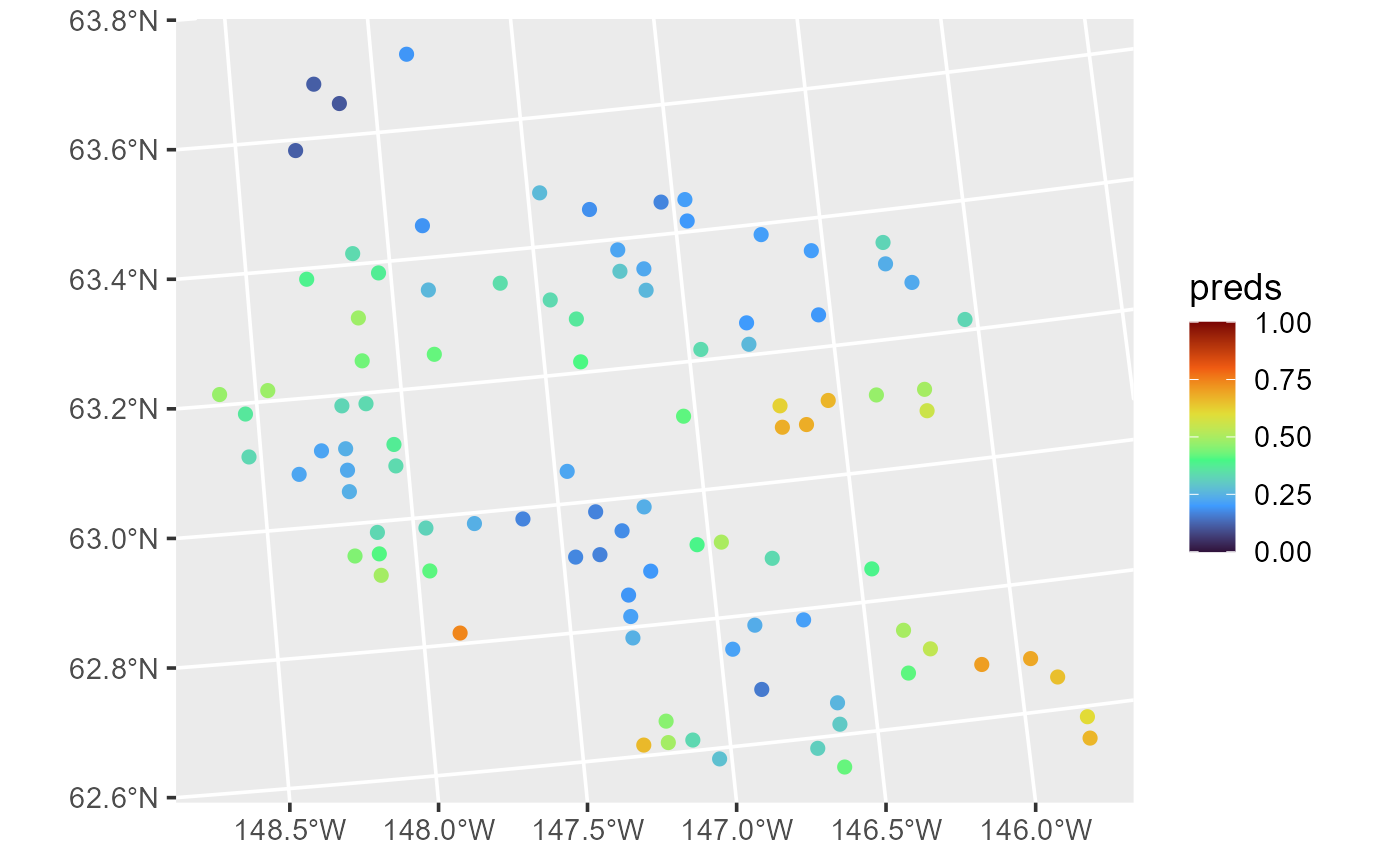

Distribution of moose presence probability predictions in Alaska.

These predictions have similar spatial patterns as moose presence the observed data. Next we remove the model predictions from moose_preds and show how augment() can be used to obtain the same predictions alongside prediction intervals (on the response scale):

moose_preds$preds <- NULL
augment(binmod, newdata = moose_preds, type = "response", interval = "prediction")

#> Simple feature collection with 100 features and 5 fields
#> Geometry type: POINT
#> Dimension:     XY
#> Bounding box:  xmin: 269386.2 ymin: 1418453 xmax: 419976.2 ymax: 1541763
#> Projected CRS: NAD83 / Alaska Albers
#> # A tibble: 100 × 6
#>     elev strat .fitted .lower .upper           geometry
#>  * <dbl> <chr>   <dbl>  <dbl>  <dbl>        <POINT [m]>
#>  1  143. L       0.705 0.248   0.946 (401239.6 1436192)
#>  2  324. L       0.336 0.0373  0.868 (352640.6 1490695)
#>  3  158. L       0.263 0.0321  0.792 (360954.9 1491590)
#>  4  221. M       0.243 0.0360  0.734 (291839.8 1466091)
#>  5  209. M       0.742 0.270   0.957 (310991.9 1441630)
#>  6  218. L       0.191 0.0196  0.736 (304473.8 1512103)
#>  7  127. L       0.179 0.0226  0.673 (339011.1 1459318)
#>  8  122. L       0.241 0.0344  0.738 (342827.3 1463452)
#>  9  191  L       0.386 0.0414  0.902 (284453.8 1502837)
#> 10  105. L       0.494 0.114   0.882 (391343.9 1483791)
#> # ℹ 90 more rows

Simulating Spatial Generalized Data

Several functions exist to simulate spatial generalized data: sprbinom() for binomial random variables; sprbeta() for beta random variables; sprpois() for Poisson random variables; sprnbinom() for negative binomial random variables; sprgamma() for gamma random variables; and spinvgauss() for inverse Gaussian random variables. All of these functions share similar syntax with sprnorm() for simulating spatial Gaussian data and require a spcov_params() object. The generalized data simulation functions work by first simulating spatial Gaussian data on the link scale. Then this realization is used as the mean by which to simulate the spatial generalized linear model data.

We recreate sim_params and sim_data by running

sim_params <- spcov_params("exponential", de = 5, ie = 1, range = 0.5)
set.seed(0)
n <- 3000
x <- runif(n)
y <- runif(n)
sim_coords <- tibble::tibble(x, y)

We simulate a Bernoulli (binomial with size one) random variable by running

sim_response <- sprbinom(sim_params, data = sim_coords, xcoord = x, ycoord = y)
sim_data <- tibble::tibble(sim_coords, sim_response = factor(sim_response))

and visualize it by running

ggplot(sim_data, aes(x = x, y = y, color = sim_response)) +
  geom_point(size = 1.5) +
  scale_color_viridis_d(option = "H") +
  theme_gray(base_size = 14)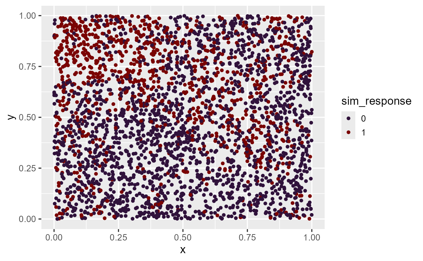

Spatial binomial data simulated in the unit square.

There is noticeable patterning in the response variable (sim_response) in the same places where there is noticeable patterning for the spatial Gaussian data. This is expected, as the spatial Gaussian data are used to inform the mean (proportion) parameter of the binomial data. Thus where the mean (proportion) parameter is higher, the more likely the binomial observation takes on the value one (successes are usually coded as a one).

Additional Examples

We previously showed how to use spmodel to model binary data via spatial binomial regression. Recall that spmodel can also be used to model count data via spatial Poisson regression or spatial negative binomial regression, proportion data via spatial beta regression, and skewed, positive data via spatial gamma regression or spatial inverse Gaussian regression. Next we provide examples of fitting a few of these models.

Poisson regression is used to model count data. To quantify the relationship between moose counts (count) and elevation, we fit a spatial Poisson regression model and make predictions by running

poismod <- spglm(count ~ elev, family = "poisson",
                 data = moose, spcov_type = "exponential")
predict(poismod, newdata = moose_preds)

Poisson regression assumes the mean and variance are equal. Often in practice, the variance is larger than the mean. When the variance is larger than the mean, there is said to be overdispersion in the data. Negative binomial regression accounts for overdispersion via an extra dispersion parameter that allows the variance to change separately from the mean (recall the full negative binomial regression parameterization is available in the technical details vignette). We fit a spatial negative binomial regression model to the moose count data and make predictions by running

nbmod <- spglm(count ~ elev, family = "nbinomial",
               data = moose, spcov_type = "exponential")
predict(nbmod, newdata = moose_preds)

Gamma regression is used to model skewed, positive data. Suppose instead of modeling the sulfate data using a spatial linear model, we modeled sulfate using spatial gamma regression. We fit a spatial gamma regression model to the sulfate data and make predictions by running

gammamod <- spglm(sulfate ~ 1, family = "Gamma",
                  data = sulfate, spcov_type = "exponential")
predict(gammamod, newdata = sulfate_preds)

Discussion

Throughout this vignette, we have shown how to use spmodel to fit, summarize, and predict for a variety of spatial statistical models. Spatial linear models for point-referenced data (i.e., geostatistical models) are fit using the splm() function while spatial linear models for areal data (i.e., spatial autoregressive models) are fit using the spautor() function. Spatial generalized linear models for point-referenced data (i.e., generalized geostatistical models) are fit using the spglm() function while spatial generalized linear models for areal data (i.e., spatial generalized autoregressive models) are fit using the spgautor() function. Several model-fit statistics and diagnostics are available. The broom functions tidy() and glance() are used to tidy and glance at a fitted model. The broom function augment() is used to augment data with model diagnostics and augment newdata with predictions. Several advanced features are available to accommodate fixed covariance parameter values, random effects, partition factors, anisotropy, simulated data, big data approximations, and random forests for model fitting and prediction.

We appreciate feedback from users regarding spmodel. To learn more about how to provide feedback or contribute to spmodel, please visit our GitHub repository at https://github.com/USEPA/spmodel.

References

Anselin, Luc, Ibnu Syabri, and Youngihn Kho. 2010. “GeoDa: An Introduction to Spatial Data Analysis.” In Handbook of Applied Spatial Analysis, 73–89. Springer.

Appelhans, Tim, Florian Detsch, Christoph Reudenbach, and Stefan Woellauer. 2022. Mapview: Interactive Viewing of Spatial Data in r. https://CRAN.R-project.org/package=mapview.

Bates, Douglas, Martin Mächler, Ben Bolker, and Steve Walker. 2015. “Fitting Linear Mixed-Effects Models Using lme4.” Journal of Statistical Software 67 (1): 1–48. https://doi.org/10.18637/jss.v067.i01.

Box, George EP, and David R Cox. 1964. “An Analysis of Transformations.” Journal of the Royal Statistical Society: Series B (Methodological) 26 (2): 211–43.

Cook, R Dennis, and Sanford Weisberg. 1982. Residuals and Influence in Regression. New York: Chapman; Hall.

Cressie, Noel. 1985. “Fitting Variogram Models by Weighted Least Squares.” Journal of the International Association for Mathematical Geology 17 (5): 563–86.

———. 1993. Statistics for Spatial Data. John Wiley & Sons.

Curriero, Frank C, and Subhash Lele. 1999. “A Composite Likelihood Approach to Semivariogram Estimation.” Journal of Agricultural, Biological, and Environmental Statistics, 9–28.

Fox, Eric W, Jay M Ver Hoef, and Anthony R Olsen. 2020. “Comparing Spatial Regression to Random Forests for Large Environmental Data Sets.” PloS One 15 (3): e0229509.

Harville, David A. 1977. “Maximum Likelihood Approaches to Variance Component Estimation and to Related Problems.” Journal of the American Statistical Association 72 (358): 320–38.

Hastie, Trevor, Robert Tibshirani, Jerome H Friedman, and Jerome H Friedman. 2009. The Elements of Statistical Learning: Data Mining, Inference, and Prediction. Vol. 2. Springer.

MacQueen, J. 1967. “Classification and Analysis of Multivariate Observations.” In 5th Berkeley Symp. Math. Statist. Probability, 281–97. University of California Los Angeles LA USA.

Montgomery, Douglas C, Elizabeth A Peck, and G Geoffrey Vining. 2021. Introduction to Linear Regression Analysis. John Wiley & Sons.

Myers, Raymond H, Douglas C Montgomery, G Geoffrey Vining, and Timothy J Robinson. 2012. Generalized Linear Models: With Applications in Engineering and the Sciences. John Wiley & Sons.

Patterson, Desmond, and Robin Thompson. 1971. “Recovery of Inter-Block Information When Block Sizes Are Unequal.” Biometrika 58 (3): 545–54.

Pebesma, Edzer. 2018. “Simple Features for R: Standardized Support for Spatial Vector Data.” The R Journal 10 (1): 439–46. https://doi.org/10.32614/RJ-2018-009.

Pinheiro, José, and Douglas Bates. 2006. Mixed-Effects Models in s and s-PLUS. Springer science & business media.

Robinson, David, Alex Hayes, and Simon Couch. 2021. broom: Convert Statistical Objects into Tidy Tibbles. https://CRAN.R-project.org/package=broom.

Tobler, Waldo R. 1970. “A Computer Movie Simulating Urban Growth in the Detroit Region.” Economic Geography 46 (sup1): 234–40.

Ver Hoef, Jay M, Eryn Blagg, Michael Dumelle, Philip M Dixon, Dale L Zimmerman, and Paul Conn. 2023. “Marginal Inference for Hierarchical Generalized Linear Mixed Models with Patterned Covariance Matrices Using the Laplace Approximation.” arXiv Preprint arXiv:2305.02978.

Ver Hoef, Jay M, Michael Dumelle, Matt Higham, Erin E Peterson, and Daniel J Isaak. 2023. “Indexing and Partitioning the Spatial Linear Model for Large Data Sets.” arXiv Preprint arXiv:2305.07811.

Ver Hoef, Jay M, Erin E Peterson, Mevin B Hooten, Ephraim M Hanks, and Marie-Josèe Fortin. 2018. “Spatial Autoregressive Models for Statistical Inference from Ecological Data.” Ecological Monographs 88 (1): 36–59.

Wickham, Hadley. 2016. ggplot2: Elegant Graphics for Data Analysis. Springer-Verlag New York. https://ggplot2.tidyverse.org.

Wolfinger, Russ, Randy Tobias, and John Sall. 1994. “Computing Gaussian Likelihoods and Their Derivatives for General Linear Mixed Models.” SIAM Journal on Scientific Computing 15 (6): 1294–1310.

Appendices

An Additional Example Using `caribou`

The purpose of this example is to show more applications of the splm() and spautor() functions when the data are not an sf object, as well as to show a few other functions in spmodel. The caribou data are are designed experiment with two treatments observed on an equally spaced grid and can be analyzed as point-referenced or areal data. We view the first few rows of caribou by running

caribou

#> # A tibble: 30 × 5
#>    water tarp      z     x     y
#>    <fct> <fct> <dbl> <dbl> <dbl>
#>  1 Y     clear  2.42     1     6
#>  2 Y     shade  2.44     2     6
#>  3 Y     none   1.81     3     6
#>  4 N     clear  1.97     4     6
#>  5 N     shade  2.38     5     6
#>  6 Y     none   2.22     1     5
#>  7 N     clear  2.10     2     5
#>  8 Y     clear  1.80     3     5
#>  9 Y     shade  1.96     4     5
#> 10 Y     none   2.10     5     5
#> # ℹ 20 more rows

First we analyze caribou as point-referenced data. Because caribou is not an sf object, we must provide the columns in caribou that represent the x-coordinates and y-coordinates. We fit a spatial linear model regressing nitrogen percentage (z) on water presence (water) and tarp cover (tarp) by running

cariboumod <- splm(z ~ water + tarp, data = caribou,
                   spcov_type = "exponential", xcoord = x, ycoord = y)

An analysis of variance can be conducted to assess the overall impact of the tarp variable, which has three levels (clear, shade, and none), and the water variable, which has two levels (water and no water). We perform an analysis of variance and tidy the results by running

tidy(anova(cariboumod))

#> # A tibble: 3 × 4
#>   effects        df statistic  p.value
#>   <chr>       <int>     <dbl>    <dbl>
#> 1 (Intercept)     1     43.5  4.33e-11
#> 2 water           1      1.66 1.98e- 1
#> 3 tarp            2     15.4  4.51e- 4

There is significant evidence that at least one tarp cover impacts nitrogen. Note that, like in summary(), these p-values are associated with an asymptotic hypothesis test (here, an asymptotic Chi-squared test).

Next we analyze caribou as areal data. Because caribou is not an sf object, we must create a weights matrix. We define two observations as neighbors if they are adjacent (directly east, west, north, or south) to one another. Two observations in caribou are adjacent if the distance between them equals one (recall that observations are not neighbors with themselves):

coords <- cbind(caribou$x, caribou$y)
dists <- as.matrix(dist(coords))
W <- dists == 1

Currently, W is a logical matrix with TRUEs and FALSEs. We coerce it to a numeric matrix by running

W <- W * 1

The $ij$th value in W is 1 if the observation in the $i$th row is neighbors with the observation in the $j$th row and 0 otherwise. We fit a spatial autoregressive model regressing the nitrogen percentage (z) on water presence (water) and tarp cover (tarp) by running

cariboumod <- spautor(z ~ water + tarp, data = caribou,
                      spcov_type = "car", W = W)

We perform an analysis of variance and tidy the results by running

tidy(anova(cariboumod))

#> # A tibble: 3 × 4
#>   effects        df statistic   p.value
#>   <chr>       <int>     <dbl>     <dbl>
#> 1 (Intercept)     1    720.   1.67e-158
#> 2 water           1      1.80 1.80e-  1
#> 3 tarp            2     15.1  5.31e-  4

Random Effect Syntax

A couple of common ways to specify random effects in the random argument to splm() or spautor() include:

~ (1 | group) : Random intercepts for each level of group. ~ group is shorthand for ~ (1 | group).
~ (var | group): Random intercepts for each level of group and random slopes that depend on the variable var for each level of group.

Some additional syntax for more complicated random effects structures include:

~ (var - 1 | group): Random slopes (without intercepts) that depend on the variable var for each level of group.
~ (1 | group:subgroup): Random intercepts for each combination of levels in group and levels in subgroup. ~ group:subgroup is shorthand for ~ (1 | group:subgroup).
~ (var | group:subgroup): Random intercepts for each combination of levels in group and levels in subgroup and random slopes that depend on the variable var for each combination of levels in group and levels in subgroup.
~ (var - 1 | group:subgroup): Random slopes (without intercepts) that depend on the variable var for each combination of levels in group and levels in subgroup.
~ (1 | group/subgroup): Shorthand for ~ (1 | group) + (1 | group:subgroup). Commonly, the group/subgroup notation implies subgroup is nested within group.
~ (var | group/subgroup): Shorthand for ~ (var | group) + (var | group:subgroup). Commonly, the group/subgroup notation implies subgroup is nested within group.
~ (var - 1 | group/subgroup): Shorthand for ~ (var - 1 | group) + (var - 1 | group:subgroup). Commonly, the group/subgroup notation implies subgroup is nested within group.

Distinct random effects terms are separated in random by +. Each term must be wrapped in parentheses. For example, to incorporate random intercepts for group and subgroup, random looks like ~ (1 | group) + (1 | subgroup). For random intercepts, recall that ~ group is shorthand for ~ (1 | group). Thus, an equivalent representation of ~ (1 | group) + (1 | subgroup) is ~ group + subgroup. Note that for both random intercepts and random slopes, the variable on the right-hand side of | (i.e., group, subgroup, group:subgroup) must be a factor (or character) variable.

Michael Dumelle, Matt Higham, and Jay M. Ver Hoef

Introduction

The Spatial Linear Model

Model Fitting

Estimation

Model-Fit Statistics

Diagnostics

The broom functions: tidy(), glance(), and augment()

An Areal Data Example

Prediction

Advanced Features

Fixing Spatial Covariance Parameters

Fitting and Predicting for Multiple Models

Random Effects

Partition Factors

Anisotropy

Simulating Spatial Data

Big Data

Model Fitting

Prediction

Random Forest Spatial Residual Models

Spatial Generalized Linear Models

Model Fitting

Prediction

Simulating Spatial Generalized Data

Additional Examples

Discussion

References

Appendices

An Additional Example Using caribou

Random Effect Syntax

The broom functions: `tidy()`, `glance()`, and `augment()`

An Additional Example Using `caribou`