8 A SPGLM Application to the “Dancer” Damselfly (Argia)
Throughout this section, we will use the following packages:

To start this exercise, we’ll introduce a new R package called finsyncR. This package was developed by US EPA scientists and academic collaborators.

From the finsyncR GitHub page:
(fish and invertebrate synchronizer in R) is a data management package that integrates and processes national-level aquatic biomonitoring datasets in the U.S., with a focus on fish and macroinvertebrates sampled in rivers and streams.
The sources of data for this package are the United States Environmental Protection Agency’s (USEPA) National Aquatic Resource Surveys (NARS), namely the National River and Streams Assessment (NRSA), and United States Geological Survey’s (USGS) BioData.
In short, finsyncR provides us with access to thousands of biological samples across the U.S. from both EPA and USGS sources (e.g., Rumschlag et al. 2023). We’ll be using EPA data today. The EPA data are from the National Aquatic Resources Assessment’s Wadeable Streams Assessment (2001-2004) and National Rivers and Streams Assessments (NRSA; 2008/2009, 2013/2014, and 2018/2019).
We encourage potential users of finsyncR to thoroughly read the GitHub tutorial and other associated materials. A paper describing the package is currently under review in Methods in Ecology and Evolution.
8.1 Data Prep
8.1.1 Biological (Dependent) Data
Next, we will use finsyncR to get genus-level macroinvert data from just EPA and rarefy to 300 count. The code will also convert the data to occurrence data (1 = detect, 0 = non-detect) and set a seed to make it reproducible. Finally, we will include samples from boatable streams rather than just those that are wadeable.
macros <- getInvertData(dataType = "occur",
taxonLevel = "Genus",
agency = "EPA",
lifestage = FALSE,
rarefy = TRUE,
rarefyCount = 300,
sharedTaxa = FALSE,
seed = 1,
boatableStreams = T)
#>
finsyncR is running: Gathering, joining, and cleaning EPA raw data
finsyncR is running: Rarefying EPA data
finsyncR is running: Applying taxonomic fixes to EPA data
finsyncR is running: Finalizing data for output
finsyncR data synchronization complete
print(dim(macros))
#> [1] 6174 856
# Print an example of the data
kable(macros[1:5, 1:23])| Agency | SampleID | ProjectLabel | SiteNumber | CollectionDate | CollectionYear | CollectionMonth | CollectionDayOfYear | Latitude_dd | Longitude_dd | CoordinateDatum | COMID | StreamOrder | WettedWidth | PredictedWettedWidth_m | NARS_Ecoregion | SampleTypeCode | AreaSampTot_m2 | FieldSplitRatio | LabSubsamplingRatio | PropID | Gen_ID_Prop | Ablabesmyia |
|---|---|---|---|---|---|---|---|---|---|---|---|---|---|---|---|---|---|---|---|---|---|---|
| EPA | 10000 | NRSA0809 | NRS_KS-10018 | 2008-08-05 | 2008 | 8 | 218 | 39.01491 | -98.01046 | NAD83 | 18865370 | 2 | 2.2525 | 2.68 | SPL | BERWW | 1.022 | NA | NA | 1.0000000 | 0.9373650 | 1 |
| EPA | 10001 | NRSA0809 | NRS_KS-10008 | 2008-08-11 | 2008 | 8 | 224 | 37.39528 | -98.92628 | NAD83 | 21012349 | 3 | 4.9850 | 5.37 | SPL | BERWW | 0.372 | NA | NA | 0.1770852 | 0.8576998 | 0 |
| EPA | 10004 | NRSA0809 | NRS_KS-10040 | 2008-07-15 | 2008 | 7 | 197 | 37.78662 | -96.42997 | NAD83 | 21515712 | 4 | 10.0800 | 9.05 | TPL | BERWW | 1.022 | NA | NA | 0.4374453 | 0.9310987 | 1 |
| EPA | 10006 | NRSA0809 | NRS_KS-10064 | 2008-08-25 | 2008 | 8 | 238 | 37.99323 | -99.32134 | NAD83 | 22082845 | 7 | 4.5150 | 9.18 | SPL | BERWW | 0.186 | NA | NA | 0.2187705 | 0.9659091 | 0 |
| EPA | 1002013 | NRSA1314 | NRS_KS-10126 | 2013-04-30 | 2013 | 4 | 120 | 39.12843 | -95.65402 | NAD83 | 3645992 | 2 | 5.5500 | 5.18 | TPL | BERW | 1.022 | NA | NA | 0.2916983 | 0.9026718 | 0 |
Let’s massage the table with dplyr to get what we want, including data on the occurences of Argia:
- Select columns of interest, including the Argia occurrence column.
- Remove data related to the EPA’s Wadeable Streams Assessment (2001-2004).
- Convert “CollectionDate” to a date (
lubridate::date()) and convert presence/absence to a factor. - Finally, convert table to a
sfobject and transform to EPSG:5070.
# Flexible code so we could model another taxon
genus <- 'Argia'
taxon <- macros %>%
dplyr::select(SampleID,
ProjectLabel,
CollectionDate,
Latitude_dd,
Longitude_dd,
all_of(genus)) %>%
mutate(CollectionDate = date(CollectionDate),
presence =
as.factor(pull(., genus))) %>%
st_as_sf(coords = c('Longitude_dd', 'Latitude_dd'), crs = 4269) %>%
st_transform(crs = 5070)To visualize the data, we will read in a layer of lower 48 states to give some context. To do this we can use the tigris package. We will also remove non-conterminous states and transform the projection to our favorite - EPSG:5070.
First, let’s plot the observed presences/absences in the data…
ggplot() +
geom_sf(data = states, fill = NA) +
geom_sf(data = taxon,
aes(color = presence),
size = 1.5,
alpha = 0.65) +
scale_color_manual(values=c("#d9d9d9", "#08519c")) +
theme_bw() +
theme(legend.position="bottom") 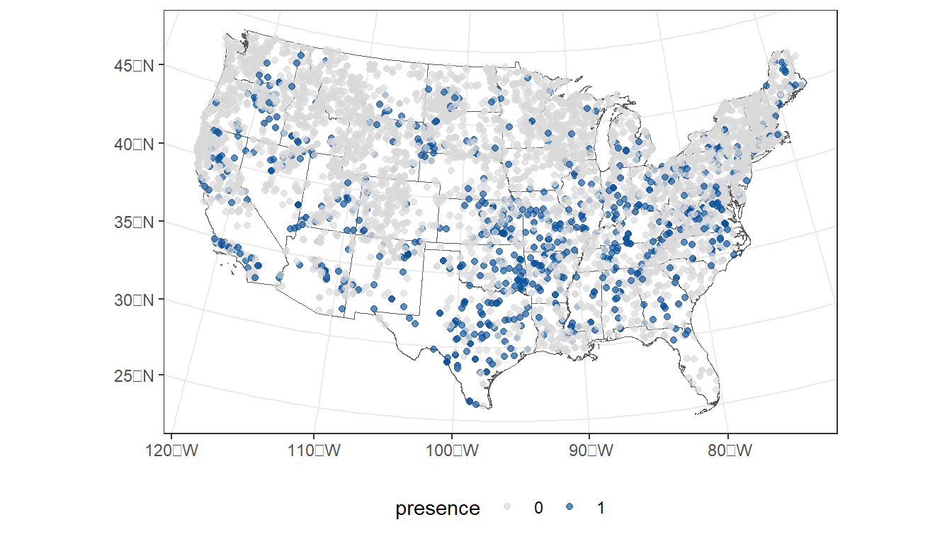
…and by NRSA survey period:
ggplot() +
geom_sf(data = states, fill = NA) +
geom_sf(data = taxon,
aes(color = ProjectLabel),
size = 1.5,
alpha = 0.75) +
scale_color_manual(values=c("#a6cee3", "#1f78b4", "#b2df8a", "#33a02c")) +
theme_bw() +
theme(legend.position="bottom") 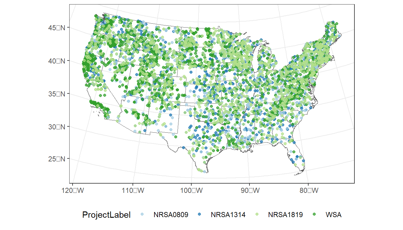
For today’s exercise, we’ll narrow down the samples to the northeaster region of the U.S.
- Select states from the northeaster U.S.
- Select NRSA sample sites that intersect with these states.
- Filter to just the 2013/2014 and 2018/2019 sample periods.
- Create a new column for sample year.
- Select desired columns.
# Filter to study region (states)
region <- states %>%
filter(STUSPS %in% c('VT', 'NH', 'ME', 'NY', 'RI',
'MA', 'CT', 'NJ', 'PA', 'DE'))
# Use region as spatial filter (sf::st_filter()) for taxon of interest
taxon_rg <- taxon %>%
st_filter(region) %>%
filter(ProjectLabel %in% c('NRSA1314', 'NRSA1819')) %>%
mutate(year = year(ymd(CollectionDate))) %>%
select(SampleID:CollectionDate, presence:year)
ggplot() +
geom_sf(data = region, fill = NA) +
geom_sf(data = taxon_rg,
aes(color = presence)) +
scale_color_manual(values=c("#d9d9d9", "#08519c")) +
theme_bw() +
theme(legend.position="bottom") 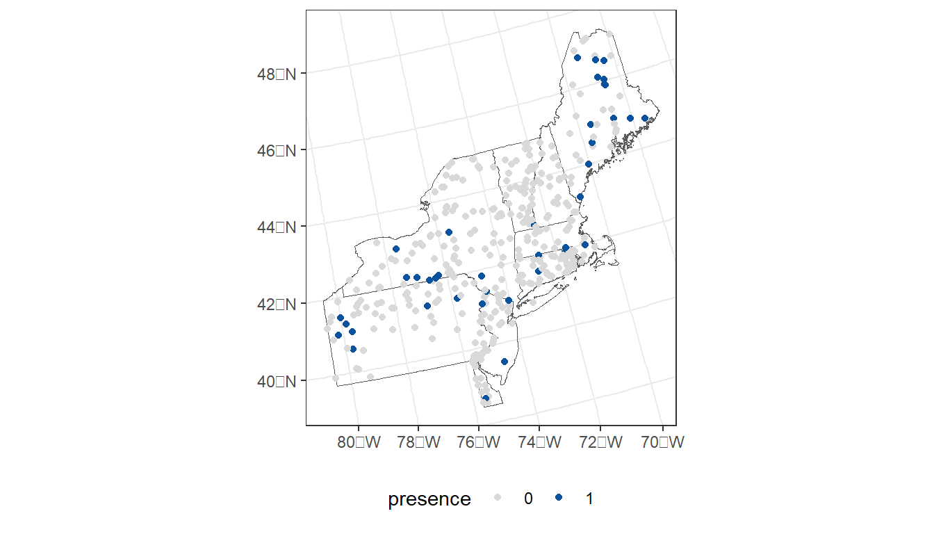
ggplot() +
geom_sf(data = region, fill = NA) +
geom_sf(data = taxon_rg,
aes(color = ProjectLabel)) +
scale_color_manual(values=c("#1f78b4", "#b2df8a")) +
theme_bw() +
theme(legend.position="bottom") 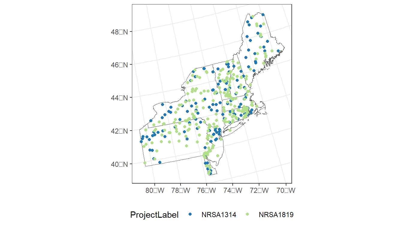
8.1.2 Predictor (Independent) Data
- Obtain list of NHDPlus COMIDs that match sample sites from
nhdplusTools
- Use NLDI service via StreamCat to get the COMIDs
- Create a vector of COMIDs by splitting the COMID string
- Add COMID to our Argia occurrence table
comids <- sc_get_comid(taxon_rg)
#comids <- read_rds('./data/nrsa_comids.rds')
comid_vect <-
comids %>%
str_split(',') %>%
unlist() %>%
as.integer()
taxon_rg <-
taxon_rg %>%
mutate(COMID = comid_vect) - Get non-varying StreamCat data.
sc <-
sc_get_data(comid = comids,
aoi = 'watershed',
metric = 'bfi, precip8110, wetindex, elev',
showAreaSqKm = TRUE)- Get year-specific wetlands within watersheds.
- NLCD contains data on the distribution of herbaceous (pcthbwet) and woody (pctwdwet) wetlands. We will combine them into a single metric representing the % of the watershed comprised of wetlands.
- Duplicate the data, but offset by 1 year so we can 2019 NLCD to 2018 observations (same for 2013 NLCD and 2014 NRSA).
wetlands <-
sc_get_data(comid = comids,
aoi = 'watershed',
metric = 'pctwdwet2013,pcthbwet2013,pctwdwet2019,pcthbwet2019',
showAreaSqKm = FALSE) %>%
# Sum wetland types to create single wetlands metric
mutate(PCTWETLAND2013WS = PCTHBWET2013WS + PCTWDWET2013WS,
PCTWETLAND2019WS = PCTHBWET2019WS + PCTWDWET2019WS) %>%
# Reduce columns
select(COMID, PCTWETLAND2013WS, PCTWETLAND2019WS) %>%
# Create long table w/ column name w/out year
pivot_longer(!COMID, names_to = 'tmpcol', values_to = 'PCTWETLANDXXXXWS') %>%
# Create new column of year by removing "PCTWETLAND" and "WS" from names
mutate(year = as.integer(str_replace_all(tmpcol, 'PCTWETLAND|WS', '')))
# But some samples have 2014 and 2018 as sample years? How can we trick the data into joining?
# We can match 2019 data to 2018 observations by subtracting a year and appending it to the data
# Create tmp table with 1 added or subtracted to year of record
tmp_wetlands <- wetlands %>%
mutate(year = ifelse(year == 2013, year + 1, year - 1))
# rbind() wetlands and tmp_wetlands so we have records to join to 2014 and 2018
wetlands <- wetlands %>%
rbind(tmp_wetlands) %>%
select(-tmpcol)- Year-specific impervious surfaces within 100-m riparian buffer.
riparian_imp <-
sc_get_data(comid = comids,
aoi = 'riparian_watershed',
metric = 'pctimp2013, pctimp2019',
showAreaSqKm = FALSE) %>%
select(-WSAREASQKMRP100) %>%
pivot_longer(!COMID, names_to = 'tmpcol', values_to = 'PCTIMPXXXXWSRP100') %>%
mutate(year = as.integer(
str_replace_all(tmpcol, 'PCTIMP|WSRP100', '')))
tmp_imp <- riparian_imp %>%
mutate(year = ifelse(year == 2013, year + 1, year - 1))
riparian_imp <- riparian_imp %>%
rbind(tmp_imp) %>%
select(-tmpcol)- PRISM air temperatures for sample periods
- The
prismpackage requires that we set a temporary folder in our work space. Here, we set it to “prism_data” inside of our “data” folder. It will create this folder if it does not already exist. - We then stack the climate rasters and use
terra::extract()to
# Get these years of PRISM
years <- c(2013, 2014, 2018, 2019)
# Set the PRISM directory (creates directory in not present)
prism_set_dl_dir("./data/prism_data", create = TRUE)
# Download monthly PRISM rasters (tmean)
get_prism_monthlys('tmean',
years = years,
mon = 7:8,
keepZip = FALSE)
#>
|
| | 0%
|
|======== | 12%
|
|================= | 25%
|
|========================= | 38%
|
|================================== | 50%
|
|========================================== | 62%
|
|================================================== | 75%
|
|=========================================================== | 88%
|
|===================================================================| 100%
# Create stack of downloaded PRISM rasters
tmn <- pd_stack((prism_archive_subset("tmean","monthly",
years = years,
mon = 7:8)))
# Extract tmean at sample points and massage data
tmn <- terra::extract(tmn,
# Transform taxon_rg to CRS of PRISM on the fly
taxon_rg %>%
st_transform(crs = st_crs(tmn))) %>%
# Add COMIDs to extracted values
data.frame(COMID = comid_vect, .) %>%
# Remove front and back text from PRISM year/month in names
rename_with( ~ stringr::str_replace_all(., 'PRISM_tmean_stable_4kmM3_|_bil', '')) %>%
# Pivot to long table and calle column TMEANPRISMXXXXPT, XXXX indicates year
pivot_longer(!COMID, names_to = 'year_month',
values_to = 'TMEANPRISMXXXXPT') %>%
# Create new column of year
mutate(year = year(ym(year_month))) %>%
# Average July and August temperatures
summarise(TMEANPRISMXXXXPT = mean(TMEANPRISMXXXXPT, na.rm = TRUE),
.by = c(COMID, year))8.1.3 Combine Dependent and Independent Data
argia_model_data <-
taxon_rg %>%
left_join(sc, join_by(COMID)) %>%
left_join(wetlands, join_by(COMID, year)) %>%
left_join(riparian_imp, join_by(COMID, year)) %>%
left_join(tmn, join_by(COMID, year)) %>%
drop_na()
cor(argia_model_data %>%
st_drop_geometry() %>%
select(WSAREASQKM:TMEANPRISMXXXXPT))
#> WSAREASQKM ELEVWS WETINDEXWS BFIWS
#> WSAREASQKM 1.00000000 0.19649723 -0.0844127 -0.17679333
#> ELEVWS 0.19649723 1.00000000 -0.6020139 -0.56349466
#> WETINDEXWS -0.08441270 -0.60201389 1.0000000 0.40544326
#> BFIWS -0.17679333 -0.56349466 0.4054433 1.00000000
#> PRECIP8110WS -0.15455456 -0.02973549 -0.1213487 0.17231568
#> PCTWETLANDXXXXWS -0.13274790 -0.53982414 0.7838752 0.49003820
#> PCTIMPXXXXWSRP100 -0.10603160 -0.39811621 0.1008221 0.07181972
#> TMEANPRISMXXXXPT 0.08241251 -0.68038439 0.3688678 0.25976247
#> PRECIP8110WS PCTWETLANDXXXXWS PCTIMPXXXXWSRP100
#> WSAREASQKM -0.15455456 -0.13274790 -0.10603160
#> ELEVWS -0.02973549 -0.53982414 -0.39811621
#> WETINDEXWS -0.12134865 0.78387523 0.10082210
#> BFIWS 0.17231568 0.49003820 0.07181972
#> PRECIP8110WS 1.00000000 0.03862313 0.17634436
#> PCTWETLANDXXXXWS 0.03862313 1.00000000 -0.04885782
#> PCTIMPXXXXWSRP100 0.17634436 -0.04885782 1.00000000
#> TMEANPRISMXXXXPT 0.04030682 0.24384288 0.43121267
#> TMEANPRISMXXXXPT
#> WSAREASQKM 0.08241251
#> ELEVWS -0.68038439
#> WETINDEXWS 0.36886778
#> BFIWS 0.25976247
#> PRECIP8110WS 0.04030682
#> PCTWETLANDXXXXWS 0.24384288
#> PCTIMPXXXXWSRP100 0.43121267
#> TMEANPRISMXXXXPT 1.000000008.2 Modeling occurrence of genus Argia
8.2.1 Model formulation
formula <-
presence ~
I(log10(WSAREASQKM)) +
ELEVWS +
WETINDEXWS +
BFIWS +
PRECIP8110WS +
PCTWETLANDXXXXWS +
PCTIMPXXXXWSRP100 +
TMEANPRISMXXXXPT
bin_mod <- spglm(formula = formula,
data = argia_model_data,
family = 'binomial',
spcov_type = 'none')
bin_spmod <- spglm(formula = formula,
data = argia_model_data,
family = 'binomial',
spcov_type = 'exponential')
glances(bin_mod, bin_spmod)
#> # A tibble: 2 × 10
#> model n p npar value AIC AICc logLik deviance pseudo.r.squared
#> <chr> <int> <dbl> <int> <dbl> <dbl> <dbl> <dbl> <dbl> <dbl>
#> 1 bin_s… 550 9 3 1394. 1400. 1400. -697. 201. 0.110
#> 2 bin_m… 550 9 1 1409. 1411. 1411. -704. 342. 0.145
summary(bin_spmod)
#>
#> Call:
#> spglm(formula = formula, family = "binomial", data = argia_model_data,
#> spcov_type = "exponential")
#>
#> Deviance Residuals:
#> Min 1Q Median 3Q Max
#> -1.4692 -0.4226 -0.2762 -0.1450 2.4044
#>
#> Coefficients (fixed):
#> Estimate Std. Error z value Pr(>|z|)
#> (Intercept) 8.089431 6.729301 1.202 0.2293
#> I(log10(WSAREASQKM)) 0.808323 0.202435 3.993 6.52e-05 ***
#> ELEVWS -0.006700 0.002643 -2.535 0.0112 *
#> WETINDEXWS 0.003059 0.004851 0.631 0.5283
#> BFIWS -0.032951 0.042665 -0.772 0.4399
#> PRECIP8110WS -0.003344 0.002894 -1.156 0.2478
#> PCTWETLANDXXXXWS -0.016386 0.048407 -0.339 0.7350
#> PCTIMPXXXXWSRP100 0.088456 0.047796 1.851 0.0642 .
#> TMEANPRISMXXXXPT -0.348964 0.149201 -2.339 0.0193 *
#> ---
#> Signif. codes: 0 '***' 0.001 '**' 0.01 '*' 0.05 '.' 0.1 ' ' 1
#>
#> Pseudo R-squared: 0.1101
#>
#> Coefficients (exponential spatial covariance):
#> de ie range
#> 3.121e+00 9.212e-03 3.636e+04
#>
#> Coefficients (Dispersion for binomial family):
#> dispersion
#> 18.2.2 Model performance
# Function to convert from log odds to probability
to_prob <- function(x) exp(x)/(1+exp(x))
loocv_mod <- loocv(bin_mod, cv_predict = TRUE, se.fit = TRUE)
prob_mod <- to_prob(loocv_mod$cv_predict)
sefit_mod <- loocv_mod$se.fit
loocv_spmod <- loocv(bin_spmod, cv_predict = TRUE, se.fit = TRUE)
prob_spmod <- to_prob(loocv_spmod$cv_predict)
sefit_spmod <- loocv_spmod$se.fit
pROC::auc(argia_model_data$presence, prob_mod)
#> Area under the curve: 0.7908
pROC::auc(argia_model_data$presence, prob_spmod)
#> Area under the curve: 0.9154
argia_model_data <- argia_model_data %>%
mutate(prob_spmod = prob_spmod,
sefit_spmod = sefit_spmod)
ggplot() +
geom_sf(data = region, fill = NA) +
geom_sf(data = argia_model_data,
aes(color = prob_spmod)) +
scale_color_viridis_b() +
theme_bw() +
theme(legend.position="bottom")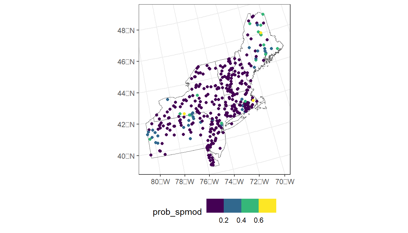
ggplot() +
geom_sf(data = region, fill = NA) +
geom_sf(data = argia_model_data,
aes(color = sefit_spmod)) +
scale_color_distiller(palette = 'Reds', direction = 1) +
theme_bw() +
theme(legend.position="bottom")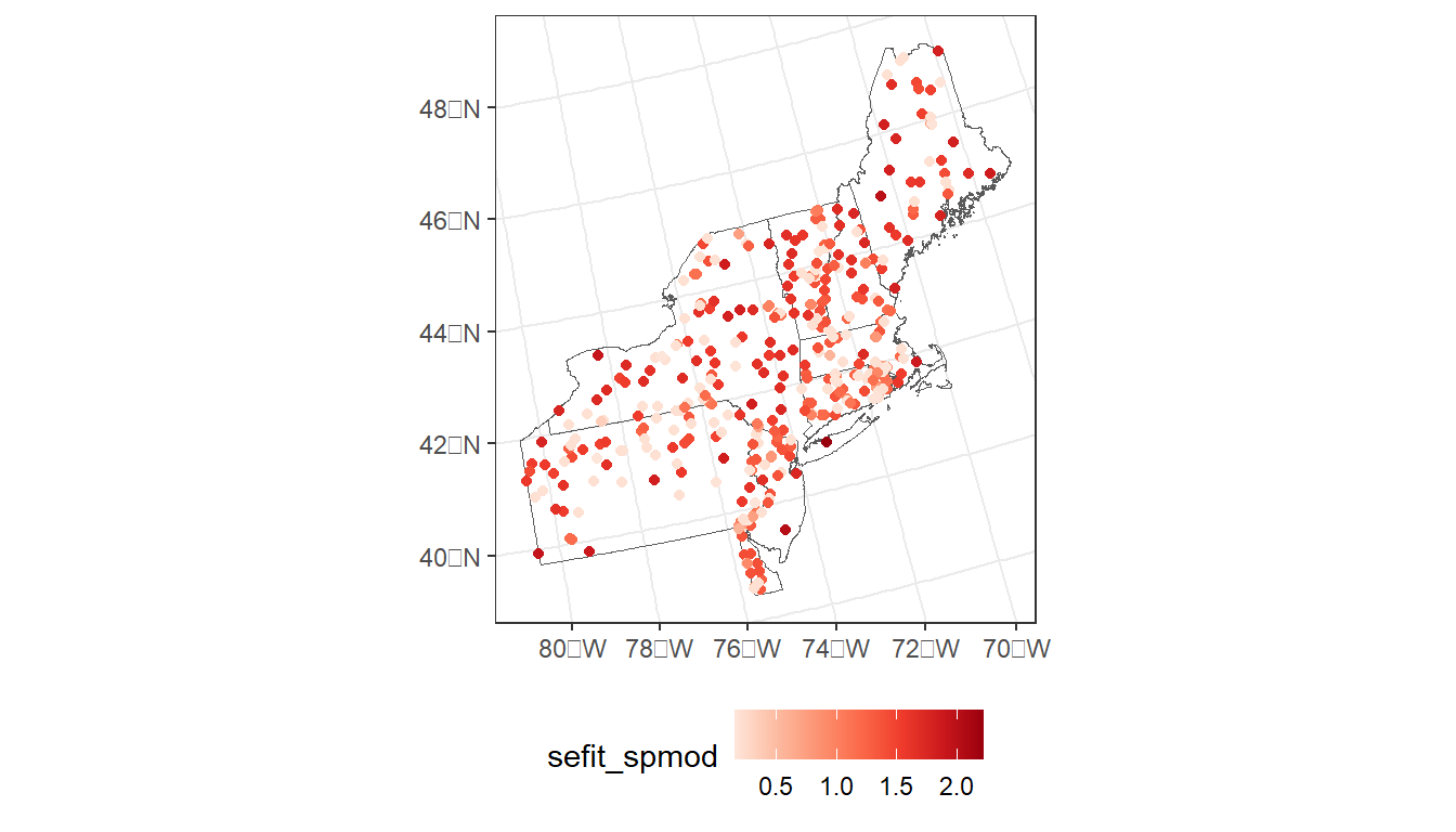
8.2.3 EXTRA: Mapping predictions
state <- region %>%
filter(STUSPS == "NJ") %>%
st_transform(crs = 4326)
# Use get_nhdplus to access the individual stream sub-catchments
pourpoints <-
nhdplusTools::get_nhdplus(AOI = state,
realization = 'outlet') |>
filter(flowdir == "With Digitized")
sc_prd <- sc_get_data(state = 'NJ',
aoi = 'watershed,riparian_watershed',
metric = 'bfi,precip8110,wetindex,elev,pctwdwet2019,pcthbwet2019,pctimp2019') |>
mutate(PCTWETLANDXXXXWS = PCTWDWET2019WS + PCTHBWET2019WS) |>
rename(PCTIMPXXXXWSRP100 = PCTIMP2019WSRP100) |>
select(COMID, WSAREASQKM, ELEVWS, WETINDEXWS, BFIWS,
PRECIP8110WS, PCTWETLANDXXXXWS, PCTIMPXXXXWSRP100)
tmn_prd <-
pd_stack((prism_archive_subset("tmean","monthly",
years = 2019,
mon = 7:8)))
tmn_prd <-
terra::extract(tmn_prd,
pourpoints %>%
st_transform(crs = st_crs(tmn_prd))) |>
as.tibble() |>
mutate(COMID = pourpoints$comid,
TMEANPRISMXXXXPT = (PRISM_tmean_stable_4kmM3_201907_bil + PRISM_tmean_stable_4kmM3_201908_bil)/2) |>
select(COMID, TMEANPRISMXXXXPT)
argia_pred_data <- sc_prd |>
left_join(tmn_prd, join_by(COMID)) |>
left_join(pourpoints, join_by(COMID == comid)) |>
st_as_sf() |>
st_transform(crs = 5070) |>
select(COMID, WSAREASQKM, ELEVWS, WETINDEXWS,
BFIWS, PRECIP8110WS, PCTWETLANDXXXXWS,
PCTIMPXXXXWSRP100, TMEANPRISMXXXXPT) |>
na.omit()
argia_predict <-
augment(bin_spmod,
newdata = argia_pred_data,
type = 'response',
se_fit = TRUE,
local = TRUE)
ggplot() +
geom_sf(data = argia_predict,
aes(color = .fitted),
size = 0.9) +
scale_color_distiller(palette = 'YlOrRd', direction = 2) +
theme_bw()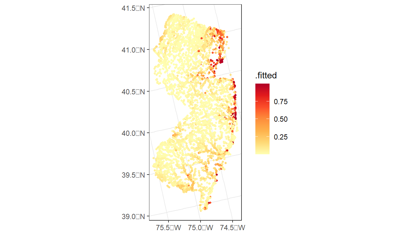
ggplot() +
geom_sf(data = argia_predict,
aes(color = .se.fit),
size = 0.9) +
scale_color_distiller(palette = 'YlOrRd', direction = 2) +
theme_bw()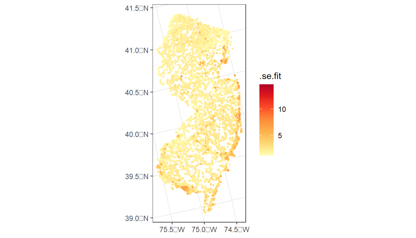
8.3 R Code Appendix
library(finsyncR)
library(tidyverse)
library(sf)
library(tigris)
library(StreamCatTools)
library(nhdplusTools)
library(spmodel)
library(data.table)
library(pROC)
library(knitr)
library(prism)
macros <- getInvertData(dataType = "occur",
taxonLevel = "Genus",
agency = "EPA",
lifestage = FALSE,
rarefy = TRUE,
rarefyCount = 300,
sharedTaxa = FALSE,
seed = 1,
boatableStreams = T)
print(dim(macros))
# Print an example of the data
kable(macros[1:5, 1:23])
# Flexible code so we could model another taxon
genus <- 'Argia'

taxon <- macros %>%
  dplyr::select(SampleID,
                ProjectLabel,
                CollectionDate,
                Latitude_dd,
                Longitude_dd,
                all_of(genus))  %>%
  mutate(CollectionDate = date(CollectionDate),
         presence =
           as.factor(pull(., genus)))  %>%
  st_as_sf(coords = c('Longitude_dd', 'Latitude_dd'), crs = 4269)  %>%
  st_transform(crs = 5070)
states <- tigris::states(cb = TRUE, progress_bar = FALSE)  %>%
  filter(!STUSPS %in% c('HI', 'PR', 'AK', 'MP', 'GU', 'AS', 'VI'))  %>%
  st_transform(crs = 5070)
ggplot() +
  geom_sf(data = states, fill = NA) +
  geom_sf(data = taxon,
          aes(color = presence),
          size = 1.5,
          alpha = 0.65) +
  scale_color_manual(values=c("#d9d9d9", "#08519c")) +
  theme_bw() +
  theme(legend.position="bottom")
ggplot() +
  geom_sf(data = states, fill = NA) +
  geom_sf(data = taxon,
          aes(color = ProjectLabel),
          size = 1.5,
          alpha = 0.75) +
  scale_color_manual(values=c("#a6cee3", "#1f78b4", "#b2df8a", "#33a02c")) +
  theme_bw() +
  theme(legend.position="bottom")
# Filter to study region (states)
region <- states %>%
  filter(STUSPS %in% c('VT', 'NH', 'ME', 'NY', 'RI',
                       'MA', 'CT', 'NJ', 'PA', 'DE'))

# Use region as spatial filter (sf::st_filter()) for taxon of interest
taxon_rg <- taxon %>%
  st_filter(region) %>%
  filter(ProjectLabel %in% c('NRSA1314', 'NRSA1819')) %>%
  mutate(year = year(ymd(CollectionDate))) %>%
  select(SampleID:CollectionDate, presence:year)

ggplot() +
  geom_sf(data = region, fill = NA) +
  geom_sf(data = taxon_rg,
          aes(color = presence)) +
  scale_color_manual(values=c("#d9d9d9", "#08519c")) +
  theme_bw() +
  theme(legend.position="bottom")
ggplot() +
  geom_sf(data = region, fill = NA) +
  geom_sf(data = taxon_rg,
          aes(color = ProjectLabel)) +
  scale_color_manual(values=c("#1f78b4", "#b2df8a")) +
  theme_bw() +
  theme(legend.position="bottom")
taxon_rg %>%
pull(presence) %>%
table()
comids <- sc_get_comid(taxon_rg)

#comids <- read_rds('./data/nrsa_comids.rds')
comid_vect <-
  comids %>%
  str_split(',') %>%
  unlist() %>%
  as.integer()

taxon_rg <-
  taxon_rg %>%
  mutate(COMID = comid_vect)
sc <-
  sc_get_data(comid = comids,
              aoi = 'watershed',
              metric = 'bfi, precip8110, wetindex, elev',
              showAreaSqKm = TRUE)
wetlands <-
  sc_get_data(comid = comids,
              aoi = 'watershed',
              metric = 'pctwdwet2013,pcthbwet2013,pctwdwet2019,pcthbwet2019',
              showAreaSqKm = FALSE) %>%

  # Sum wetland types to create single wetlands metric
  mutate(PCTWETLAND2013WS = PCTHBWET2013WS + PCTWDWET2013WS,
         PCTWETLAND2019WS = PCTHBWET2019WS + PCTWDWET2019WS) %>%

  # Reduce columns
  select(COMID, PCTWETLAND2013WS, PCTWETLAND2019WS) %>%

  # Create long table w/ column name w/out year
  pivot_longer(!COMID, names_to = 'tmpcol', values_to = 'PCTWETLANDXXXXWS') %>%

  # Create new column of year by removing "PCTWETLAND" and "WS" from names
  mutate(year = as.integer(str_replace_all(tmpcol, 'PCTWETLAND|WS', '')))

# But some samples have 2014 and 2018 as sample years? How can we trick the data into joining?
# We can match 2019 data to 2018 observations by subtracting a year and appending it to the data

# Create tmp table with 1 added or subtracted to year of record
tmp_wetlands <- wetlands %>%
  mutate(year = ifelse(year == 2013, year + 1, year - 1))

# rbind() wetlands and tmp_wetlands so we have records to join to 2014 and 2018
wetlands <- wetlands %>%
  rbind(tmp_wetlands) %>%
  select(-tmpcol)
riparian_imp <-
  sc_get_data(comid = comids,
              aoi = 'riparian_watershed',
              metric = 'pctimp2013, pctimp2019',
              showAreaSqKm = FALSE) %>%
  select(-WSAREASQKMRP100) %>%
  pivot_longer(!COMID, names_to = 'tmpcol', values_to = 'PCTIMPXXXXWSRP100') %>%
  mutate(year = as.integer(
    str_replace_all(tmpcol, 'PCTIMP|WSRP100', '')))

tmp_imp <- riparian_imp %>%
  mutate(year = ifelse(year == 2013, year + 1, year - 1))

riparian_imp <- riparian_imp %>%
  rbind(tmp_imp) %>%
  select(-tmpcol)
# Get these years of PRISM
years <- c(2013, 2014, 2018, 2019)
# Set the PRISM directory (creates directory in not present)
prism_set_dl_dir("./data/prism_data", create = TRUE)
# Download monthly PRISM rasters (tmean)
get_prism_monthlys('tmean',
years = years,
mon = 7:8,
keepZip = FALSE)
# Create stack of downloaded PRISM rasters
tmn <- pd_stack((prism_archive_subset("tmean","monthly",
years = years,
mon = 7:8)))
# Extract tmean at sample points and massage data
tmn <- terra::extract(tmn,
# Transform taxon_rg to CRS of PRISM on the fly
taxon_rg %>%
st_transform(crs = st_crs(tmn))) %>%
# Add COMIDs to extracted values
data.frame(COMID = comid_vect, .) %>%
# Remove front and back text from PRISM year/month in names
rename_with( ~ stringr::str_replace_all(., 'PRISM_tmean_stable_4kmM3_|_bil', '')) %>%
# Pivot to long table and calle column TMEANPRISMXXXXPT, XXXX indicates year
pivot_longer(!COMID, names_to = 'year_month',
values_to = 'TMEANPRISMXXXXPT') %>%
# Create new column of year
mutate(year = year(ym(year_month))) %>%
# Average July and August temperatures
summarise(TMEANPRISMXXXXPT = mean(TMEANPRISMXXXXPT, na.rm = TRUE),
.by = c(COMID, year))
argia_model_data <-
taxon_rg %>%
left_join(sc, join_by(COMID)) %>%
left_join(wetlands, join_by(COMID, year)) %>%
left_join(riparian_imp, join_by(COMID, year)) %>%
left_join(tmn, join_by(COMID, year)) %>%
drop_na()
cor(argia_model_data %>%
st_drop_geometry() %>%
select(WSAREASQKM:TMEANPRISMXXXXPT))
formula <-
presence ~
I(log10(WSAREASQKM)) +
ELEVWS +
WETINDEXWS +
BFIWS +
PRECIP8110WS +
PCTWETLANDXXXXWS +
PCTIMPXXXXWSRP100 +
TMEANPRISMXXXXPT
bin_mod <- spglm(formula = formula,
data = argia_model_data,
family = 'binomial',
spcov_type = 'none')
bin_spmod <- spglm(formula = formula,
data = argia_model_data,
family = 'binomial',
spcov_type = 'exponential')
glances(bin_mod, bin_spmod)
summary(bin_spmod)
# Function to convert from log odds to probability
to_prob <- function(x) exp(x)/(1+exp(x))
loocv_mod <- loocv(bin_mod, cv_predict = TRUE, se.fit = TRUE)
prob_mod <- to_prob(loocv_mod$cv_predict)
sefit_mod <- loocv_mod$se.fit
loocv_spmod <- loocv(bin_spmod, cv_predict = TRUE, se.fit = TRUE)
prob_spmod <- to_prob(loocv_spmod$cv_predict)
sefit_spmod <- loocv_spmod$se.fit
pROC::auc(argia_model_data$presence, prob_mod)
pROC::auc(argia_model_data$presence, prob_spmod)
argia_model_data <- argia_model_data %>%
mutate(prob_spmod = prob_spmod,
sefit_spmod = sefit_spmod)
ggplot() +
geom_sf(data = region, fill = NA) +
geom_sf(data = argia_model_data,
aes(color = prob_spmod)) +
scale_color_viridis_b() +
theme_bw() +
theme(legend.position="bottom")
ggplot() +
  geom_sf(data = region, fill = NA) +
  geom_sf(data = argia_model_data,
          aes(color = sefit_spmod)) +
  scale_color_distiller(palette = 'Reds', direction = 1) +
  theme_bw() +
  theme(legend.position="bottom")
state <- region %>%
  filter(STUSPS == "NJ") %>%
  st_transform(crs = 4326)

# Use get_nhdplus to access the individual stream sub-catchments
pourpoints <-
  nhdplusTools::get_nhdplus(AOI = state,
                            realization = 'outlet') |>
  filter(flowdir == "With Digitized")

sc_prd <- sc_get_data(state = 'NJ',
                      aoi = 'watershed,riparian_watershed',
                      metric = 'bfi,precip8110,wetindex,elev,pctwdwet2019,pcthbwet2019,pctimp2019') |>
  mutate(PCTWETLANDXXXXWS = PCTWDWET2019WS + PCTHBWET2019WS) |>
  rename(PCTIMPXXXXWSRP100 = PCTIMP2019WSRP100) |>
  select(COMID, WSAREASQKM, ELEVWS, WETINDEXWS, BFIWS,
         PRECIP8110WS, PCTWETLANDXXXXWS, PCTIMPXXXXWSRP100)

tmn_prd <-
  pd_stack((prism_archive_subset("tmean","monthly",
                                 years = 2019,
                                 mon = 7:8)))
tmn_prd <-
  terra::extract(tmn_prd,
                 pourpoints %>%
                   st_transform(crs = st_crs(tmn_prd))) |>
  as.tibble() |>
  mutate(COMID = pourpoints$comid,
         TMEANPRISMXXXXPT = (PRISM_tmean_stable_4kmM3_201907_bil + PRISM_tmean_stable_4kmM3_201908_bil)/2) |>
  select(COMID, TMEANPRISMXXXXPT)

argia_pred_data <- sc_prd |>
  left_join(tmn_prd, join_by(COMID)) |>
  left_join(pourpoints, join_by(COMID == comid)) |>
  st_as_sf() |>
  st_transform(crs = 5070) |>
  select(COMID, WSAREASQKM, ELEVWS, WETINDEXWS,
         BFIWS, PRECIP8110WS, PCTWETLANDXXXXWS,
         PCTIMPXXXXWSRP100, TMEANPRISMXXXXPT) |>
  na.omit()

argia_predict <-
  augment(bin_spmod,
          newdata = argia_pred_data,
          type = 'response',
          se_fit = TRUE,
          local = TRUE)

ggplot() +
  geom_sf(data = argia_predict,
          aes(color = .fitted),
          size = 0.9) +
  scale_color_distiller(palette = 'YlOrRd', direction = 2) +
  theme_bw()
ggplot() +
  geom_sf(data = argia_predict,
          aes(color = .se.fit),
          size = 0.9) +
  scale_color_distiller(palette = 'YlOrRd', direction = 2) +
  theme_bw()