5  Watershed Delineation in R

Throughout this section, we will use the following packages:

library(tidyverse)
library(sf)
library(mapview)
library(nhdplusTools)
library(FedData)
library(terra)
library(tidyterra)
library(tictoc)

We will cover accessing geospatial metrics from StreamCat and LakeCat to use as covariates in analyses. However, these data sources may not have all of the metrics you might wish to use.

For example, StreamCat/LakeCat do not include an extensive number of climate metrics beyond the long-term PRISM normals. In such cases, generating custom metrics for watersheds may be desirable.

A first step to generating custom watershed metrics is watershed delineation. The watershed boundary can then be used as a “cookie cutter” to extract statistics from other geospatial layers within the watershed’s borders.

In the past, watershed delineation in a GIS with digital elevation models (DEM) involved multiple steps, such as DEM reconditioning to remove pits and the calculation of a flow direction raster from this conditioned DEM.

Today, there are at least two online services which can be used to generate watersheds in the conterminous U.S. In this excercise, we’ll also show an example of how to extract data from a raster dataset by using the watershed as a “cookie cutter.”

5.1 USGS StreamStats

The USGS’s StreamStats is an online service and map interface that allows users to navigate to a desired location and delineate a watershed boundary with the click of a mouse:

https://streamstats.usgs.gov/ss/

In addition to the map interface, the data are also accessible via an API:

https://streamstats.usgs.gov/docs/streamstatsservices

For example, it is possible to replicate the point and click website by pasting a URL into the browser by combining the following information:

• Base service URL
• State where watershed is located
• Longitude
• Latitude
• Additional options

StreamStats delineates a basin from pre-processed DEMs based on these inputs to the service.

We can write a custom function to make this request. This code:

• Combines the required inputs into a single text query
• Massages the data returned by the API to create a sf object

# Create custom function to delineate watershed from StreamStats service
streamstats_ws = function(state, longitude, latitude){
  p1 = 'https://streamstats.usgs.gov/streamstatsservices/watershed.geojson?rcode='
  p2 = '&xlocation='
  p3 = '&ylocation='
  p4 = '&crs=4269&includeparameters=false&includeflowtypes=false&includefeatures=true&simplify=true'
  query <-  paste0(p1, state, p2, toString(longitude), p3, toString(latitude), p4)
  mydata <- jsonlite::fromJSON(query, simplifyVector = FALSE, simplifyDataFrame = FALSE)
  poly_geojsonsting <- jsonlite::toJSON(mydata$featurecollection[[2]]$feature, auto_unbox = TRUE)
  poly <- geojsonio::geojson_sf(poly_geojsonsting) 
  poly
}

# Define location for delineation (Calapooia Watershed)
state <- 'OR'
latitude <- 44.62892
longitude <- -123.13113

# Delineate watershed
cal_ws <- streamstats_ws('OR', longitude, latitude) %>% 
  st_transform(crs = 5070)

# Generate point for plotting
cal_pt <- data.frame(ptid = 'Calapooia River', lon = longitude, lat = latitude)  %>% 
  st_as_sf(coords = c('lon', 'lat'), crs = 4269) %>% 
  st_transform(crs = 5070)

cal_map <- ggplot() + 
  geom_sf(data = cal_ws, fill=NA) +
  geom_sf(data = cal_pt, size=3) +
  theme_bw()

cal_map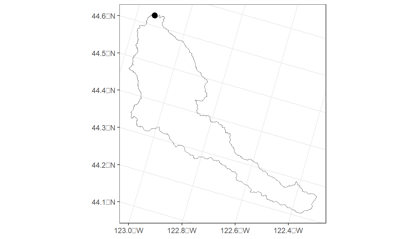

As noted above, we can replicate the call to the API by pasting the p1 to p4 + state and lat/lon:

state <- 'OR'
latitude <- 44.62892
longitude <- -123.13113

p1 = 'https://streamstats.usgs.gov/streamstatsservices/watershed.geojson?rcode='
p2 = '&xlocation='
p3 = '&ylocation='
p4 = '&crs=4269&includeparameters=false&includeflowtypes=false&includefeatures=true&simplify=true'

query <-  paste0(p1, state, p2, toString(longitude), p3, toString(latitude), p4)

print(query)
#> [1] "https://streamstats.usgs.gov/streamstatsservices/watershed.geojson?rcode=OR&xlocation=-123.13113&ylocation=44.62892&crs=4269&includeparameters=false&includeflowtypes=false&includefeatures=true&simplify=true"

However, when the query is provided to the browser, it does not look like a watershed. The additional lines of code in the function we defined above used the jsonlite and geojsonio packages to massage the output and produce the sf spatial object cal_ws.

This code produces a watershed boundary (cal_ws) for the Calapooia watershed in Oregon. But what if the latitude/longitude are slightly off of the stream network?

# A close, but different watershed
latitude <- 44.61892
longitude <- -123.13731

trib_ws <- streamstats_ws('OR', longitude, latitude) %>% 
  st_transform(crs = 5070)

trib_pt <- data.frame(ptid = 'Calapooia Trib', lon = longitude, lat = latitude)  %>% 
  st_as_sf(coords = c('lon', 'lat'), crs = 4269) %>% 
  st_transform(crs = 5070)

cal_map <- cal_map +
  geom_sf(data = trib_ws, fill=NA, color='red') +
  geom_sf(data = trib_pt, size=3, color = 'pink') 

cal_map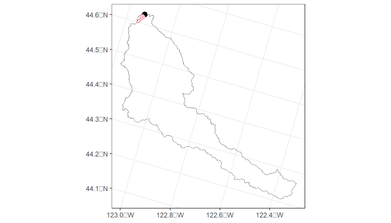

Let’s zoom into the problem. To do this we’ll use the mapview package. Here, we use mapview::mapview() to create an interactive map of the Calapooia watersheds.

mapview::mapviewOptions(fgb=FALSE)

mapview(cal_ws, alpha.regions=.08) + 
  mapview(cal_pt, col.regions = 'black') + 
  mapview(trib_ws, alpha.regions=.08, col.regions = 'red') +
  mapview(trib_pt, col.regions = 'red')  

We can see that the second lat/lon delineated a very small watershed that appears to be a tributary to the mainstem of the Calapooia. This highlights one of the challenges of watershed delineation - small discrepancies in lat/lon can produce a vastely different boundary.

In the next section, we’ll explore another method for watershed delineation.

5.2 nhdplusTools

nhdplusTools is an R package that can access the Network Linked Data Index (NLDI) service, which provides navigation and extraction of NHDPlus data:

https://doi-usgs.github.io/nhdplusTools/

nhdplusTools includes network navigation options as well as watershed delineation. The delineation method differs from StreamStats in that the sub-catchments are pre-staged and based on the local catchments of the NHDPlus.To delineate a basin, we must identify the starting point and the NLDI service walks the network for us to generate the watershed.

# Calapooia Watershed
latitude <- 44.62892
longitude <- -123.13113

# Simple feature option to generate point without any other attributes
cal_pt2 <- st_sfc(st_point(c(longitude, latitude)), crs = 4269)

# Identify the network location (NHDPlus common ID or COMID)
start_comid <- nhdplusTools::discover_nhdplus_id(cal_pt2)

# Combine info into list (required by NLDI basin function)
ws_source <- list(featureSource = "comid", featureID = start_comid)

cal_ws2 <- nhdplusTools::get_nldi_basin(nldi_feature = ws_source)

cal_map <- ggplot() + 
  geom_sf(data = cal_ws2, fill = NA) +
  geom_sf(data = cal_pt2) +
  theme_bw()

cal_map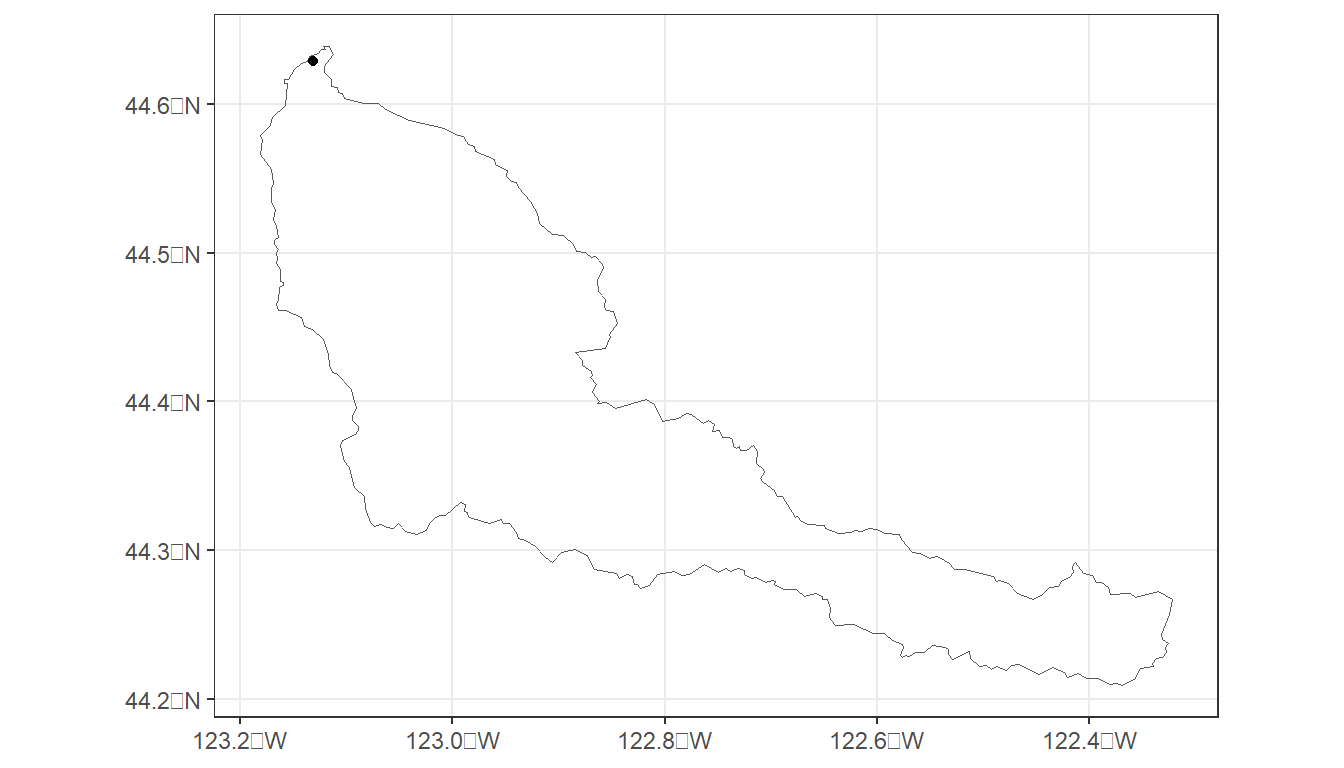

The delineated watershed should look familiar since it is the Calapooia River watershed.

However, you may notice the slight difference in the placement of the point and the outlet of the watershed relative to the StreamStats watershed.

Let’s have a closer look at the two watersheds together:

mapview::mapviewOptions(fgb=FALSE)

mapview(cal_pt, col.regions = 'black') + 
  mapview(cal_ws, alpha.regions = .08) + 
  mapview(cal_ws2, alpha.regions = .08, col.regions = 'red') 

But, what about the small tributary?

Although the points are separated by a distance, they produce the same watershed. This is because the watersheds are based the aggregation of pre-defined sub-catchments of the medium-resolution NHDPlus. Since the points fall within the same local sub-catchment, they have the same outlet and basin area.

# Trib coordinates
latitude <- 44.61892
longitude <- -123.13731

trib_pt2 <- st_sfc(st_point(c(longitude, latitude)), crs = 4269)
start_comid <- nhdplusTools::discover_nhdplus_id(trib_pt2)
ws_source <- list(featureSource = "comid", featureID = start_comid)

trib_ws2 <- nhdplusTools::get_nldi_basin(nldi_feature = ws_source)

streams <- nhdplusTools::navigate_nldi(ws_source, mode = "UT", 
                                       distance_km = 2000) %>%
  pluck('UT_flowlines')

# Use get_nhdplus to access the individual stream sub-catchments
cats <- nhdplusTools::get_nhdplus(comid = streams$nhdplus_comid,
                                  realization = 'catchment')

mapview(streams, legend = FALSE) + 
  mapview(cal_pt2, col.regions = 'red') + 
  mapview(trib_pt2, col.regions = 'blue') + 
  mapview(cal_ws2, alpha.regions=.08, col.regions = 'red') +
  mapview(cats, alpha.regions=.08, col.regions = 'blue') 

This is the major limitation of NHDPlus (and by extension StreamCat). Thus, when deciding whether to use StreamStats or NHDPlusTools for watershed delineation, it is important to consider that:

• StreamStats can delineate smaller tributaries, but cannot do large watersheds that cross state lines.

• StreamStats is not available for all U.S. states.

• NHDPlusTools can delineate smallish to large watersheds (e.g., Mississippi River), but misses very small systems. (However, you can try experimenting with their implementation of high-res NHDPlus.)

Outside of the U.S., these tools are not available. However, it is still possible to delineate a custom watershed from raw DEM data with help from the whitebox R package. This book by J.P. Gannon has instructions on how to prepare a DEM and provide catchment pourpoints for delineation.

Finally, Jeff Hollister (U.S. EPA) developed an R package called elevatr that can access DEM data from the web both within and outside the U.S.

Let’s put it all together…

Exercise

1. Delineate the Logan River watershed in Utah at -111.855, 41.707.

2. Use the watershed boundary to download NLCD land cover data.

3. Plot the NLCD data within the watershed bounday.

4. Calculate the percent cover of each land use.

Exercise Solution

tic()

# Logan River Watershed
latitude <- 41.707
longitude <- -111.855

# Define the lat/lon
start_point <- st_sfc(st_point(c(longitude, latitude)), crs = 4269)

# Find COMID of this point
start_comid <- nhdplusTools::discover_nhdplus_id(start_point)

# Create a list object that defines the feature source and starting COMID
ws_source <- list(featureSource = "comid", featureID = start_comid)

# Delineate basin
logan_ws <- nhdplusTools::get_nldi_basin(nldi_feature = ws_source) %>%

  # Transform to EPSG 5070
  st_transform(crs = 5070)

# Alternate method
# logan_ws <- streamstats_ws('UT', longitude, latitude) %>% 
#   st_transform(crs = 5070)

nlcd <- get_nlcd(
  template = logan_ws,
  year = 2021,
  label = 'Logan') %>%
  
  # Project raster to EPSG 5070
  terra::project('epsg:5070', method = 'near') %>% 
  
  # Mask the raster
  terra::mask(logan_ws) %>% 
  
  # Clip the raster
  terra::crop(logan_ws)

ggplot() + 
  geom_spatraster(data = nlcd) +
  geom_sf(data = logan_ws,
          fill = NA,
          lwd = 1.5,
          color = 'white') +
  theme_bw()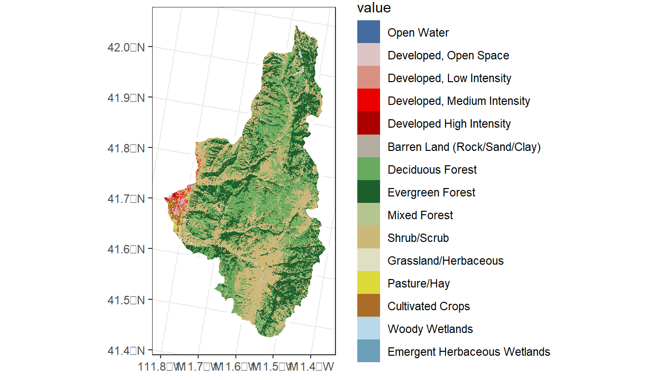

logan_nlcd <- terra::extract(nlcd, 
                             terra::vect(logan_ws))

logan_nlcd %>% 
  group_by(Class) %>% 
  summarise(count = n()) %>% 
  mutate(percent = (count / sum(count)) * 100)
#> # A tibble: 15 × 3
#>    Class                         count  percent
#>    <fct>                         <int>    <dbl>
#>  1 Open Water                      240  0.0151 
#>  2 Developed, Open Space         24184  1.52   
#>  3 Developed, Low Intensity      12049  0.756  
#>  4 Developed, Medium Intensity    7961  0.500  
#>  5 Developed High Intensity       1872  0.118  
#>  6 Barren Land (Rock/Sand/Clay)     86  0.00540
#>  7 Deciduous Forest             441144 27.7    
#>  8 Evergreen Forest             451517 28.3    
#>  9 Mixed Forest                  47735  3.00   
#> 10 Shrub/Scrub                  568734 35.7    
#> 11 Grassland/Herbaceous           9819  0.616  
#> 12 Pasture/Hay                    8310  0.522  
#> 13 Cultivated Crops              13686  0.859  
#> 14 Woody Wetlands                 5218  0.328  
#> 15 Emergent Herbaceous Wetlands    605  0.0380

toc()
#> 13.29 sec elapsed

In the exercise above, we delineated a watershed from a latitude/longitude, transformed its projection, downloaded land cover raster data for the watershed, transformed its projection, masked and clipped the raster for mapping, and calculated the percent of each land cover type within the watershed boundary – all under 30 seconds.

5.3 R Code Appendix

library(tidyverse)
library(sf)
library(mapview)
library(nhdplusTools)
library(FedData)
library(terra)
library(tidyterra)
library(tictoc)
# Create custom function to delineate watershed from StreamStats service
streamstats_ws = function(state, longitude, latitude){
  p1 = 'https://streamstats.usgs.gov/streamstatsservices/watershed.geojson?rcode='
  p2 = '&xlocation='
  p3 = '&ylocation='
  p4 = '&crs=4269&includeparameters=false&includeflowtypes=false&includefeatures=true&simplify=true'
  query <-  paste0(p1, state, p2, toString(longitude), p3, toString(latitude), p4)
  mydata <- jsonlite::fromJSON(query, simplifyVector = FALSE, simplifyDataFrame = FALSE)
  poly_geojsonsting <- jsonlite::toJSON(mydata$featurecollection[[2]]$feature, auto_unbox = TRUE)
  poly <- geojsonio::geojson_sf(poly_geojsonsting) 
  poly
}

# Define location for delineation (Calapooia Watershed)
state <- 'OR'
latitude <- 44.62892
longitude <- -123.13113

# Delineate watershed
cal_ws <- streamstats_ws('OR', longitude, latitude) %>% 
  st_transform(crs = 5070)

# Generate point for plotting
cal_pt <- data.frame(ptid = 'Calapooia River', lon = longitude, lat = latitude)  %>% 
  st_as_sf(coords = c('lon', 'lat'), crs = 4269) %>% 
  st_transform(crs = 5070)

cal_map <- ggplot() + 
  geom_sf(data = cal_ws, fill=NA) +
  geom_sf(data = cal_pt, size=3) +
  theme_bw()

cal_map
state <- 'OR'
latitude <- 44.62892
longitude <- -123.13113

p1 = 'https://streamstats.usgs.gov/streamstatsservices/watershed.geojson?rcode='
p2 = '&xlocation='
p3 = '&ylocation='
p4 = '&crs=4269&includeparameters=false&includeflowtypes=false&includefeatures=true&simplify=true'

query <-  paste0(p1, state, p2, toString(longitude), p3, toString(latitude), p4)

print(query)
# A close, but different watershed
latitude <- 44.61892
longitude <- -123.13731

trib_ws <- streamstats_ws('OR', longitude, latitude) %>% 
  st_transform(crs = 5070)

trib_pt <- data.frame(ptid = 'Calapooia Trib', lon = longitude, lat = latitude)  %>% 
  st_as_sf(coords = c('lon', 'lat'), crs = 4269) %>% 
  st_transform(crs = 5070)

cal_map <- cal_map +
  geom_sf(data = trib_ws, fill=NA, color='red') +
  geom_sf(data = trib_pt, size=3, color = 'pink') 

cal_map
mapview::mapviewOptions(fgb=FALSE)

mapview(cal_ws, alpha.regions=.08) + 
  mapview(cal_pt, col.regions = 'black') + 
  mapview(trib_ws, alpha.regions=.08, col.regions = 'red') +
  mapview(trib_pt, col.regions = 'red')  
# Calapooia Watershed
latitude <- 44.62892
longitude <- -123.13113

# Simple feature option to generate point without any other attributes
cal_pt2 <- st_sfc(st_point(c(longitude, latitude)), crs = 4269)

# Identify the network location (NHDPlus common ID or COMID)
start_comid <- nhdplusTools::discover_nhdplus_id(cal_pt2)

# Combine info into list (required by NLDI basin function)
ws_source <- list(featureSource = "comid", featureID = start_comid)

cal_ws2 <- nhdplusTools::get_nldi_basin(nldi_feature = ws_source)

cal_map <- ggplot() + 
  geom_sf(data = cal_ws2, fill = NA) +
  geom_sf(data = cal_pt2) +
  theme_bw()

cal_map
mapview::mapviewOptions(fgb=FALSE)

mapview(cal_pt, col.regions = 'black') + 
  mapview(cal_ws, alpha.regions = .08) + 
  mapview(cal_ws2, alpha.regions = .08, col.regions = 'red') 
# Trib coordinates
latitude <- 44.61892
longitude <- -123.13731

trib_pt2 <- st_sfc(st_point(c(longitude, latitude)), crs = 4269)
start_comid <- nhdplusTools::discover_nhdplus_id(trib_pt2)
ws_source <- list(featureSource = "comid", featureID = start_comid)

trib_ws2 <- nhdplusTools::get_nldi_basin(nldi_feature = ws_source)

streams <- nhdplusTools::navigate_nldi(ws_source, mode = "UT", 
                                       distance_km = 2000) %>%
  pluck('UT_flowlines')

# Use get_nhdplus to access the individual stream sub-catchments
cats <- nhdplusTools::get_nhdplus(comid = streams$nhdplus_comid,
                                  realization = 'catchment')

mapview(streams, legend = FALSE) + 
  mapview(cal_pt2, col.regions = 'red') + 
  mapview(trib_pt2, col.regions = 'blue') + 
  mapview(cal_ws2, alpha.regions=.08, col.regions = 'red') +
  mapview(cats, alpha.regions=.08, col.regions = 'blue') 

tic()

# Logan River Watershed
latitude <- 41.707
longitude <- -111.855

# Define the lat/lon
start_point <- st_sfc(st_point(c(longitude, latitude)), crs = 4269)

# Find COMID of this point
start_comid <- nhdplusTools::discover_nhdplus_id(start_point)

# Create a list object that defines the feature source and starting COMID
ws_source <- list(featureSource = "comid", featureID = start_comid)

# Delineate basin
logan_ws <- nhdplusTools::get_nldi_basin(nldi_feature = ws_source) %>%

  # Transform to EPSG 5070
  st_transform(crs = 5070)

# Alternate method
# logan_ws <- streamstats_ws('UT', longitude, latitude) %>% 
#   st_transform(crs = 5070)

nlcd <- get_nlcd(
  template = logan_ws,
  year = 2021,
  label = 'Logan') %>%
  
  # Project raster to EPSG 5070
  terra::project('epsg:5070', method = 'near') %>% 
  
  # Mask the raster
  terra::mask(logan_ws) %>% 
  
  # Clip the raster
  terra::crop(logan_ws)

ggplot() + 
  geom_spatraster(data = nlcd) +
  geom_sf(data = logan_ws,
          fill = NA,
          lwd = 1.5,
          color = 'white') +
  theme_bw()

logan_nlcd <- terra::extract(nlcd, 
                             terra::vect(logan_ws))

logan_nlcd %>% 
  group_by(Class) %>% 
  summarise(count = n()) %>% 
  mutate(percent = (count / sum(count)) * 100)

toc()