7  A SPLM Application to Lake Conductivity

Conductivity is an important water quality measure and one of growing concern due to salinization of freshwater (Cañedo-Argüelles et al. 2016, Kaushal et al. 2021).

In this exercise we will model the conductivity of lakes across Minnesota. To do so, we will read in a data set of lake conductivity measurements collected as part of EPA’s National Lakes Assessment.

This analysis is based on a recent paper by Michael Dumelle and others published in the journal Spatial Statistics. The GitHub repository for this paper is also available.

7.1 Data Prep

7.1.1 Conductivity (Dependent) Data

Load required packages…

library(tidyverse)
library(sf)
library(tigris)
library(StreamCatTools)
library(spmodel)
library(data.sfs2024)

Read and prep table of lake conductivity values…

# Read in states to give some context
states <- states(cb = TRUE, progress_bar = FALSE)  %>% 
  filter(!STUSPS %in% c('HI', 'PR', 'AK', 'MP', 'GU', 'AS', 'VI'))  %>% 
  st_transform(crs = 5070)

# Read in lakes, select/massage columns, convert to spatial object
data("cond_nla_data")

# Plot sample locations
ggplot() +
  geom_sf(data = states,
          fill = NA) +
  geom_sf(data = cond_nla_data,
          aes(color = year)) +
  scale_color_manual(values=c("#a6cee3", "#1f78b4", "#b2df8a")) +
  theme_bw() +
  theme(legend.position="bottom")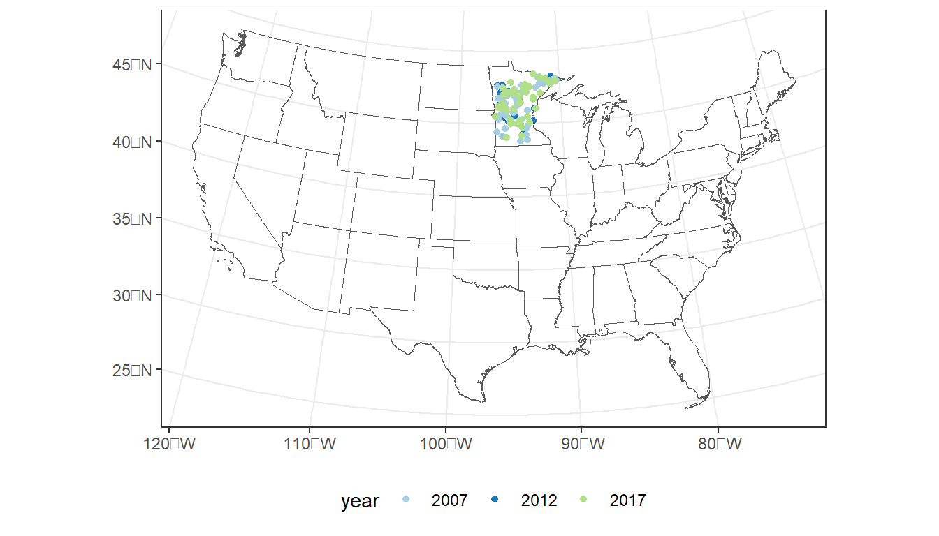 

Select sample sites within Minnesota and plot:

• Locations colored by sample year.

• Locations colored by conductivity

MN <- states %>% 
  filter(STUSPS == 'MN')

# Plot sample locations
ggplot() +
  geom_sf(data = MN,
          fill = NA) +
  geom_sf(data = cond_nla_data,
          aes(color = year)) +
  scale_color_manual(values=c("#a6cee3", "#1f78b4", "#b2df8a")) +
  theme_bw() +
  theme(legend.position="bottom")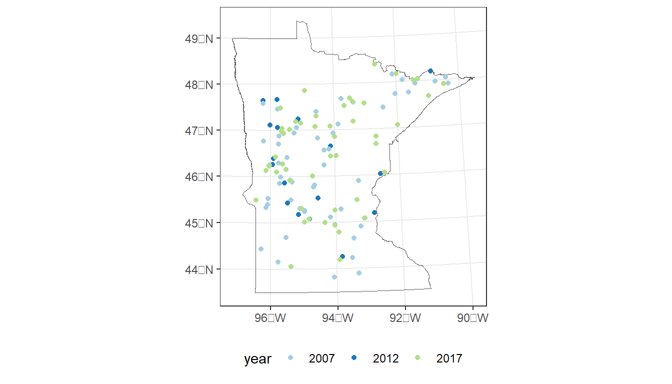 

# Plot sample locations
ggplot() +
  geom_sf(data = MN,
          fill = NA) +
  geom_sf(data = cond_nla_data,
          aes(color = log(COND_RESULT))) +
  scale_color_distiller(palette = 'YlOrRd', direction = 1) +
  theme_bw() +
  theme(legend.position="bottom")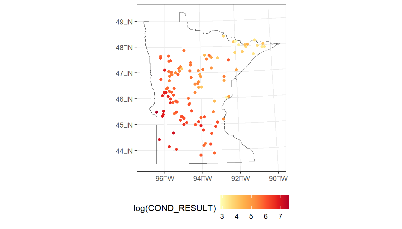 

7.1.2 LakeCat (Independent) Data

We will use the similar watershed predictors as Dumelle et al. (2023).

Already included with data table with the response variable are:

• Lake Area (AREA_HA)
• Sample year (year)

From LakeCat, we also will get the following predictor variables:

• Local long-term air temperature
• Long-term watershed precipitation
• Calcium Oxide content of underlying lithology
• Sulfur content of underlying lithology

comids <- cond_nla_data$COMID

mn_lakecat <- lc_get_data(comid = comids,
                          metric = 'Tmean8110, Precip8110,
                          CaO, S') %>% 
  select(COMID, TMEAN8110CAT, PRECIP8110WS, CAOWS, SWS)

In addition to these static LakeCat data, we would also like to pull in data from specific years of NLCD to match sample years for:

• % of watershed composed of crop area (year specific)
• % of watershed composed of urban area (year specific)

Since we have multiple years of conductivity data, we’d like to match specific years of NLCD land cover data. The years of available NLCD metrics happen to be 1 year before each NLA sample year. We’ll need to trick the tables to allow them to match and join.

This code will:

• Grab LakeCat NLCD % crop data for years 2006, 2011, 2016
• Clean and pivot columns
• Add 1 to each year since available NLCD are 1 year behind field samples

crop <- 
  
  # Grab LakeCat crop data
  lc_get_data(comid = comids,
              aoi = 'watershed',
              metric = 'pctcrop2006, pctcrop2011, pctcrop2016') %>% 
  
  # Remove watershed area from data
  select(-WSAREASQKM) %>% 
  
  # Pivot table to long to create "year" column
  pivot_longer(!COMID, names_to = 'tmpcol', values_to = 'PCTCROPWS') %>% 
  
  # Remove PCTCROP and WS to make "year" column
  mutate(year = as.integer(
    str_replace_all(tmpcol, 'PCTCROP|WS', ''))) %>% 
  
  # Add 1 to each year to match NLA years
  mutate(year = factor(year + 1)) %>% 
  
  # Remove the tmp column
  select(-tmpcol)

Do the same for urban areas, but first add medium and high urban areas:

urb <- 
  lc_get_data(comid = comids,
              aoi = 'watershed',
              metric = 'pcturbmd2006, pcturbmd2011, pcturbmd2016,
              pcturbhi2006, pcturbhi2011, pcturbhi2016',
              showAreaSqKm = FALSE) %>% 
  
  # Add up medium and high urban areas
  mutate(PCTURB2006WS = PCTURBMD2006WS + PCTURBHI2006WS,
         PCTURB2011WS = PCTURBMD2011WS + PCTURBHI2011WS,
         PCTURB2016WS = PCTURBMD2016WS + PCTURBHI2016WS) %>% 
  select(COMID, PCTURB2006WS, PCTURB2011WS, PCTURB2016WS) %>% 
  pivot_longer(!COMID, names_to = 'tmpcol', values_to = 'PCTURBWS') %>% 
  mutate(year = as.integer(
    str_replace_all(tmpcol, 'PCTURB|WS', ''))) %>% 
  mutate(year = factor(year + 1)) %>% 
  select(-tmpcol)

Now, join the various tables to make our model data:

cond_model_data <- cond_nla_data %>% 
  left_join(mn_lakecat, join_by(COMID)) %>% 
  left_join(crop, join_by(COMID, year)) %>% 
  left_join(urb, join_by(COMID, year))

7.2 Modeling lake conductivity

7.2.1 Model formulation

formula <- 
  log(COND_RESULT) ~ 
  AREA_HA + 
  year + 
  TMEAN8110CAT +
  PRECIP8110WS + 
  PCTCROPWS + 
  PCTURBWS +
  CAOWS + 
  SWS

cond_mod <- splm(formula = formula,
                 data = cond_model_data,
                 spcov_type = 'none')

cond_spmod <- splm(formula = formula,
                   data = cond_model_data,
                   spcov_type = 'exponential')

glances(cond_mod, cond_spmod)
#> # A tibble: 2 × 10
#>   model      n     p  npar value   AIC  AICc logLik deviance pseudo.r.squared
#>   <chr>  <int> <dbl> <int> <dbl> <dbl> <dbl>  <dbl>    <dbl>            <dbl>
#> 1 cond_…   162    10     3  169.  175.  175.  -84.5     152.            0.527
#> 2 cond_…   162    10     1  293.  295.  295. -146.      152             0.784

summary(cond_spmod)
#> 
#> Call:
#> splm(formula = formula, data = cond_model_data, spcov_type = "exponential")
#> 
#> Residuals:
#>      Min       1Q   Median       3Q      Max 
#> -1.88665 -0.20309  0.02008  0.27049  1.16722 
#> 
#> Coefficients (fixed):
#>                Estimate Std. Error z value Pr(>|z|)    
#> (Intercept)   8.553e+00  8.679e-01   9.856  < 2e-16 ***
#> AREA_HA       2.776e-05  5.499e-05   0.505  0.61366    
#> year2012     -1.274e-01  3.257e-02  -3.912 9.14e-05 ***
#> year2017     -1.014e-01  3.849e-02  -2.634  0.00843 ** 
#> TMEAN8110CAT  4.811e-01  7.127e-02   6.750 1.48e-11 ***
#> PRECIP8110WS -8.072e-03  1.313e-03  -6.149 7.81e-10 ***
#> PCTCROPWS     5.309e-03  2.811e-03   1.889  0.05893 .  
#> PCTURBWS      1.675e-02  1.276e-02   1.313  0.18932    
#> CAOWS        -4.172e-02  2.678e-02  -1.558  0.11931    
#> SWS           1.631e+00  8.093e-01   2.015  0.04393 *  
#> ---
#> Signif. codes:  0 '***' 0.001 '**' 0.01 '*' 0.05 '.' 0.1 ' ' 1
#> 
#> Pseudo R-squared: 0.5268
#> 
#> Coefficients (exponential spatial covariance):
#>        de        ie     range 
#> 2.588e-01 1.367e-02 2.079e+04

7.2.2 Model performance

Now, let’s the leave-one-out procedure to estimate model performance and produce predicted values and standard errors.

prd_mod <- loocv(cond_mod, se.fit = TRUE, cv_predict = TRUE) 

prd_spmod <- loocv(cond_spmod, se.fit = TRUE, cv_predict = TRUE)

bind_rows(prd_mod %>% pluck('stats'),
      prd_spmod %>% pluck('stats'))
#> # A tibble: 2 × 4
#>       bias  MSPE RMSPE  cor2
#>      <dbl> <dbl> <dbl> <dbl>
#> 1 -0.00469 0.263 0.513 0.738
#> 2 -0.00600 0.133 0.364 0.867

7.2.3 Map predicted values and standard errors

# Combine predictions with model data (spatial points)
cond_model_data <-
  cond_model_data %>% 
  mutate(prd_cond = prd_spmod %>% 
           pluck('cv_predict'), 
         se_fit = prd_spmod %>% 
           pluck('se.fit'))

# Map predicted values
ggplot() +
  geom_sf(data = MN,
          fill = NA) +
  geom_sf(data = cond_model_data,
          aes(color = prd_cond)) +
  scale_color_distiller(palette = 'YlOrRd', direction = 1) +
  theme_bw() +
  theme(legend.position="bottom")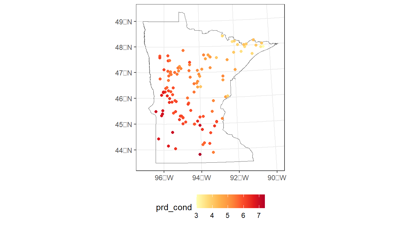 

# Map standard errors
ggplot() +
  geom_sf(data = MN,
          fill = NA) +
  geom_sf(data = cond_model_data,
          aes(color = se_fit)) +
  scale_color_distiller(palette = 'Reds', direction = 1) +
  theme_bw() +
  theme(legend.position="bottom")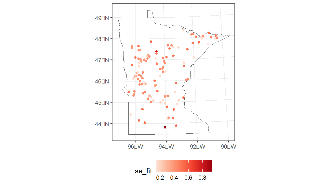 

7.3 R Code Appendix

library(tidyverse)
library(sf)
library(tigris)
library(StreamCatTools)
library(spmodel)
library(data.sfs2024)
# Read in states to give some context
states <- states(cb = TRUE, progress_bar = FALSE)  %>% 
  filter(!STUSPS %in% c('HI', 'PR', 'AK', 'MP', 'GU', 'AS', 'VI'))  %>% 
  st_transform(crs = 5070)

# Read in lakes, select/massage columns, convert to spatial object
data("cond_nla_data")

# Plot sample locations
ggplot() +
  geom_sf(data = states,
          fill = NA) +
  geom_sf(data = cond_nla_data,
          aes(color = year)) +
  scale_color_manual(values=c("#a6cee3", "#1f78b4", "#b2df8a")) +
  theme_bw() +
  theme(legend.position="bottom") 

MN <- states %>% 
  filter(STUSPS == 'MN')

# Plot sample locations
ggplot() +
  geom_sf(data = MN,
          fill = NA) +
  geom_sf(data = cond_nla_data,
          aes(color = year)) +
  scale_color_manual(values=c("#a6cee3", "#1f78b4", "#b2df8a")) +
  theme_bw() +
  theme(legend.position="bottom") 

# Plot sample locations
ggplot() +
  geom_sf(data = MN,
          fill = NA) +
  geom_sf(data = cond_nla_data,
          aes(color = log(COND_RESULT))) +
  scale_color_distiller(palette = 'YlOrRd', direction = 1) +
  theme_bw() +
  theme(legend.position="bottom") 

comids <- cond_nla_data$COMID

mn_lakecat <- lc_get_data(comid = comids,
                          metric = 'Tmean8110, Precip8110,
                          CaO, S') %>% 
  select(COMID, TMEAN8110CAT, PRECIP8110WS, CAOWS, SWS)
crop <- 
  
  # Grab LakeCat crop data
  lc_get_data(comid = comids,
              aoi = 'watershed',
              metric = 'pctcrop2006, pctcrop2011, pctcrop2016') %>% 
  
  # Remove watershed area from data
  select(-WSAREASQKM) %>% 
  
  # Pivot table to long to create "year" column
  pivot_longer(!COMID, names_to = 'tmpcol', values_to = 'PCTCROPWS') %>% 
  
  # Remove PCTCROP and WS to make "year" column
  mutate(year = as.integer(
    str_replace_all(tmpcol, 'PCTCROP|WS', ''))) %>% 
  
  # Add 1 to each year to match NLA years
  mutate(year = factor(year + 1)) %>% 
  
  # Remove the tmp column
  select(-tmpcol)
urb <- 
  lc_get_data(comid = comids,
              aoi = 'watershed',
              metric = 'pcturbmd2006, pcturbmd2011, pcturbmd2016,
              pcturbhi2006, pcturbhi2011, pcturbhi2016',
              showAreaSqKm = FALSE) %>% 
  
  # Add up medium and high urban areas
  mutate(PCTURB2006WS = PCTURBMD2006WS + PCTURBHI2006WS,
         PCTURB2011WS = PCTURBMD2011WS + PCTURBHI2011WS,
         PCTURB2016WS = PCTURBMD2016WS + PCTURBHI2016WS) %>% 
  select(COMID, PCTURB2006WS, PCTURB2011WS, PCTURB2016WS) %>% 
  pivot_longer(!COMID, names_to = 'tmpcol', values_to = 'PCTURBWS') %>% 
  mutate(year = as.integer(
    str_replace_all(tmpcol, 'PCTURB|WS', ''))) %>% 
  mutate(year = factor(year + 1)) %>% 
  select(-tmpcol)
cond_model_data <- cond_nla_data %>% 
  left_join(mn_lakecat, join_by(COMID)) %>% 
  left_join(crop, join_by(COMID, year)) %>% 
  left_join(urb, join_by(COMID, year))
formula <- 
  log(COND_RESULT) ~ 
  AREA_HA + 
  year + 
  TMEAN8110CAT +
  PRECIP8110WS + 
  PCTCROPWS + 
  PCTURBWS +
  CAOWS + 
  SWS

cond_mod <- splm(formula = formula,
                 data = cond_model_data,
                 spcov_type = 'none')

cond_spmod <- splm(formula = formula,
                   data = cond_model_data,
                   spcov_type = 'exponential')

glances(cond_mod, cond_spmod)

summary(cond_spmod)

prd_mod <- loocv(cond_mod, se.fit = TRUE, cv_predict = TRUE) 

prd_spmod <- loocv(cond_spmod, se.fit = TRUE, cv_predict = TRUE)

bind_rows(prd_mod %>% pluck('stats'),
      prd_spmod %>% pluck('stats'))


# Combine predictions with model data (spatial points)
cond_model_data <-
  cond_model_data %>% 
  mutate(prd_cond = prd_spmod %>% 
           pluck('cv_predict'), 
         se_fit = prd_spmod %>% 
           pluck('se.fit'))

# Map predicted values
ggplot() +
  geom_sf(data = MN,
          fill = NA) +
  geom_sf(data = cond_model_data,
          aes(color = prd_cond)) +
  scale_color_distiller(palette = 'YlOrRd', direction = 1) +
  theme_bw() +
  theme(legend.position="bottom") 

# Map standard errors
ggplot() +
  geom_sf(data = MN,
          fill = NA) +
  geom_sf(data = cond_model_data,
          aes(color = se_fit)) +
  scale_color_distiller(palette = 'Reds', direction = 1) +
  theme_bw() +
  theme(legend.position="bottom")