6 StreamCat & LakeCat
Throughout this section, we will use the following packages:
6.1 Why StreamCat/LakeCat?

The examples of watershed delineation and metric extraction we covered thus far have been for relatively small systems. The process to generate watershed information can be far more complicated for large watersheds, when the desired metrics are needed at many sites across a large geographic extent, or when data layers that are not served as part of other R packages.
For these reasons, we developed the StreamCat and LakeCat datasets. StreamCat uses the medium resolution NHPlus (version 2.1) as its geospatial framework to provide watershed summaries of several hundred metrics for all accumulative watersheds in the NHDPlus - about 2.6 million stream segments. Likewise, LakeCat provides watershed metrics for close to 400,000 lakes across the conterminous U.S. as well.
Both datasets are now accessible through the StreamCatTools package.
6.2 Accessing StreamCat
Let’s revisit the Calapooia watershed and extract percent row crop for 2019:
# Calapooia Watershed
latitude <- 44.62892
longitude <- -123.13113
# Make point sf of sample site
pt <- data.frame(site_name = 'Calapooia',
longitude = longitude,
latitude = latitude) %>%
st_as_sf(coords = c('longitude', 'latitude'), crs = 4269)
# Generate watershed
cal_ws <- pt %>%
nhdplusTools::discover_nhdplus_id() %>%
list(featureSource = "comid", featureID = .) %>%
nhdplusTools::get_nldi_basin() %>%
st_transform(crs = 5070)
# Download NLCD for 2019
nlcd <- get_nlcd(
template = cal_ws,
year = 2019,
label = 'Calapooia') %>%
terra::project('epsg:5070', method = 'near')
# Use terra to extract the watershed metrics
terra::extract(nlcd,
terra::vect(cal_ws)) %>%
group_by(Class) %>%
summarise(count = n()) %>%
mutate(percent = (count / sum(count)) * 100) %>%
filter(Class == 'Cultivated Crops')
#> # A tibble: 1 × 3
#> Class count percent
#> <fct> <int> <dbl>
#> 1 Cultivated Crops 112475 10.5Now let’s extract the same information using StreamCatTools.
We can find the metric name by consulting the StreamCat variable list.
I can also be useful to explore the online map and table interfaces of StreamCat.
comid <- sc_get_comid(pt)
sc_get_data(comid = comid,
metric = 'PctCrop2019',
aoi = 'watershed')
#> # A tibble: 1 × 3
#> COMID WSAREASQKM PCTCROP2019WS
#> <dbl> <dbl> <dbl>
#> 1 23763521 965. 10.5StreamCat pre-stages the calculated metrics in an online database and accessible via an API to make them available to the public.
In addition to watershed-level summaries, StreamCat provides metrics for the local catchment (i.e., the area draining to the stream segment, excluding upstream sources).
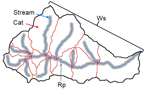
sc_get_data(comid = comid,
metric = 'PctCrop2019',
aoi = 'catchment,watershed')
#> # A tibble: 1 × 5
#> COMID WSAREASQKM CATAREASQKM PCTCROP2019CAT PCTCROP2019WS
#> <dbl> <dbl> <dbl> <dbl> <dbl>
#> 1 23763521 965. 8.49 36.6 10.5We can see the difference between the local catchment and accumulative watershed boundaries in this map.
trib_pt2 <- st_sfc(st_point(c(longitude, latitude)), crs = 4269)
start_comid <- nhdplusTools::discover_nhdplus_id(trib_pt2)
ws_source <- list(featureSource = "comid", featureID = start_comid)
trib_ws2 <- nhdplusTools::get_nldi_basin(nldi_feature = ws_source)
streams <- nhdplusTools::navigate_nldi(ws_source, mode = "UT",
distance_km = 2000) %>%
pluck('UT_flowlines')
# Use get_nhdplus to access the individual stream sub-catchments
all_catchments <- nhdplusTools::get_nhdplus(comid = streams$nhdplus_comid,
realization = 'catchment')
focal_cat <- nhdplusTools::get_nhdplus(comid = start_comid,
realization = 'catchment')
mapview(streams, color='blue', legend = FALSE) +
mapview(focal_cat, alpha.regions=.08, col.regions = 'red') +
mapview(all_catchments, alpha.regions=.08, col.regions = 'yellow') For a subset of watershed metrics, summaries within ~100m of the stream segment are also available for catchments and watersheds:
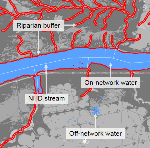
sc_get_data(comid = comid,
metric = 'PctCrop2019',
aoi = 'catchment,riparian_catchment,watershed,riparian_watershed') %>%
as.data.frame()
#> COMID WSAREASQKM WSAREASQKMRP100 CATAREASQKM CATAREASQKMRP100
#> 1 23763521 964.6101 136.17 8.4933 1.1097
#> PCTCROP2019CATRP100 PCTCROP2019WSRP100 PCTCROP2019CAT PCTCROP2019WS
#> 1 9.08 8.4 36.59 10.49StreamCatTools also makes it very easy to grab data for entire regions. In this example, we will extract % crop for the entire state of Iowa and plot these percentages as a histogram.
iowa_crop <- sc_get_data(state = 'IA',
metric = 'PctCrop2019',
aoi = 'watershed')
ggplot() +
geom_histogram(data = iowa_crop,
aes(x = PCTCROP2019WS)) +
theme_bw()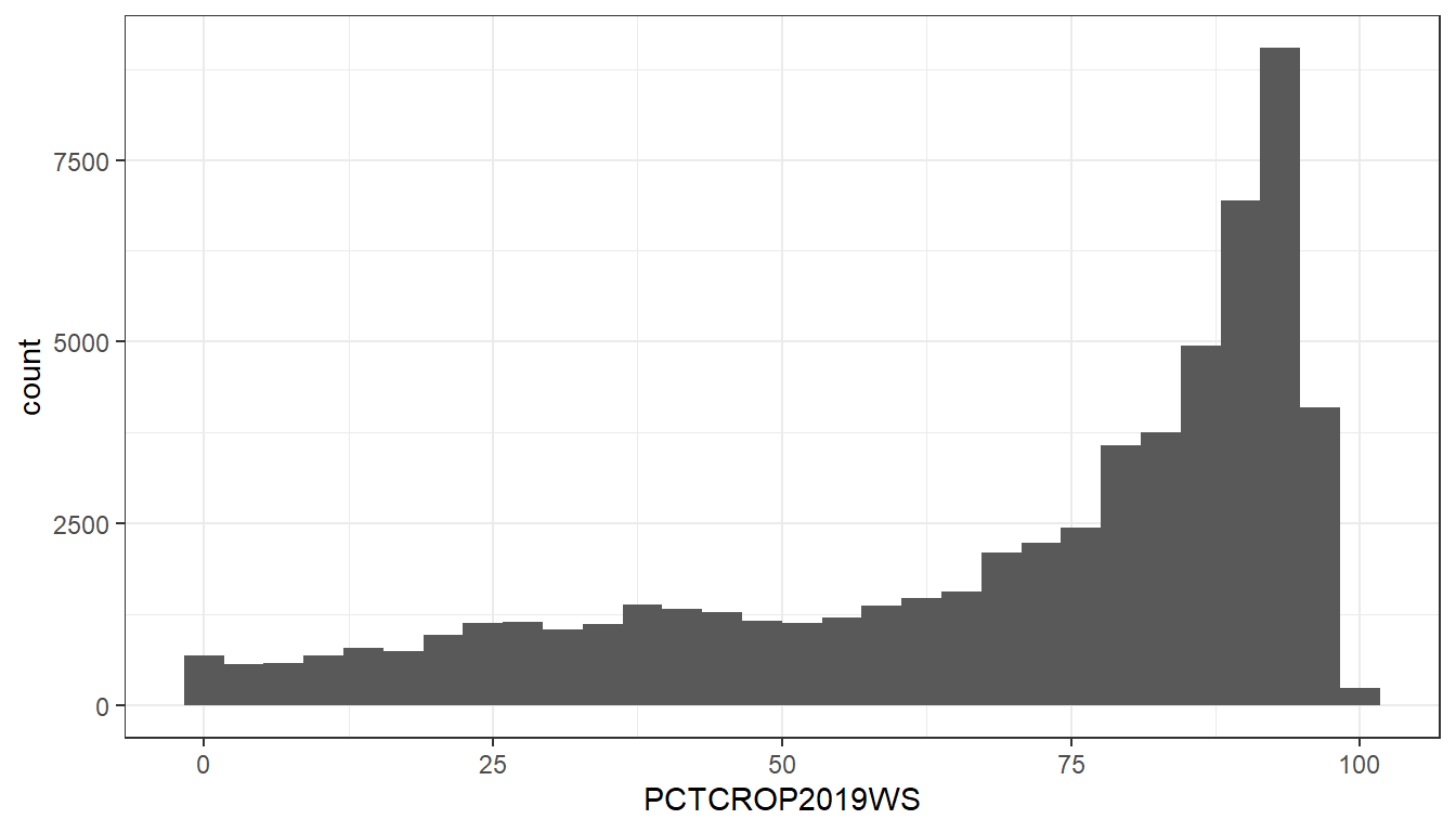
We can provide multiple metrics to the request by separating them with a comma.
Note that the request is provided as a single string, 'PctCrop2001, PctCrop2019', rather than a vector of metrics: c('PctCrop2001', 'PctCrop2019'). However, the request itself is agnostic to formatting of the text. For example, these requests will also work: 'pctcrop2001, pctcrop2019' or 'PCTCROP2001,PCTCROP2019'.
Here, we compare % watershed crop in 2001 to 2019:
iowa_crop <- sc_get_data(state = 'IA',
metric = 'PctCrop2001, PctCrop2019',
aoi = 'watershed')
# Pivot table to long format
iowa_crop_long <- iowa_crop %>%
pivot_longer(
cols = !COMID:WSAREASQKM,
values_to = 'PctCrop',
names_to = 'Year')
ggplot() +
geom_boxplot(data = iowa_crop_long,
aes(x = Year,
y = PctCrop)) +
theme_bw()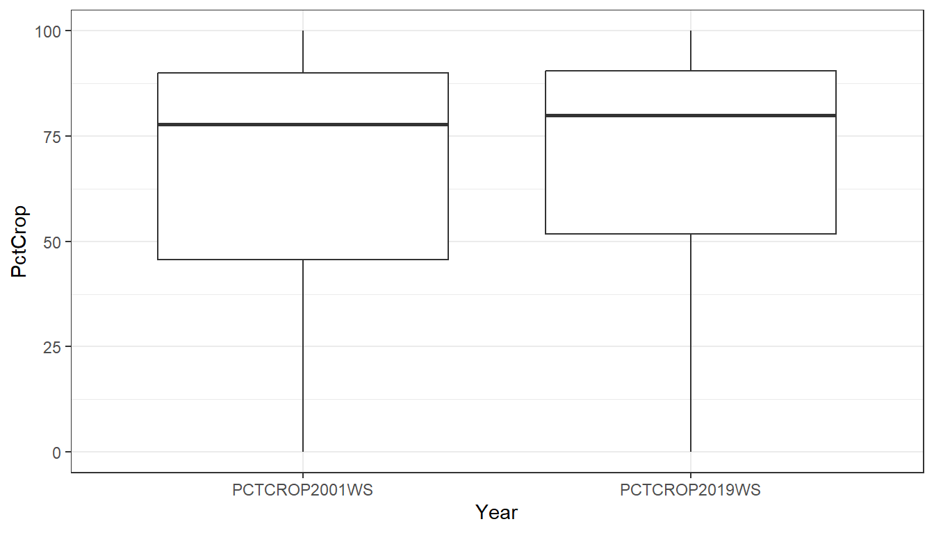
StreamCat contains hundreds of metrics and we recommend consulting the metric list to identify those of interest for your study.
6.3 Accessing LakeCat
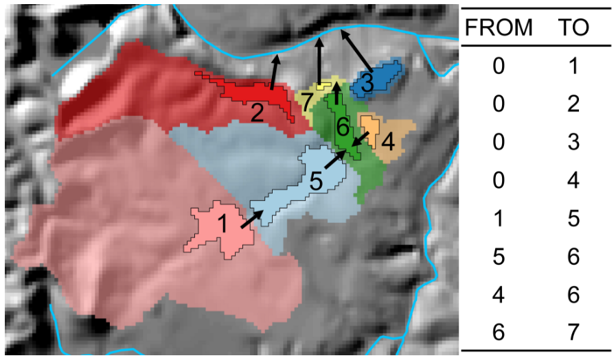
Like StreamCat, LakeCat makes local catchment and watershed metrics available for lakes across the lower 48 states. Like StreamCat, the metrics were developed from a framework of pre-staged lake-catchments that allowed for accumulation of results, even when lakes are nested.
The challenge of watershed delineation and extraction of data is even greater than for lakes than streams. There are no online services that do this. Therefore, LakeCat is one of the only ways to get watershed metrics for lakes (however, see LAGOS-NE and LAGOS-US GEO).
 As with StreamCat, the Metrics and Definitions page is the best way to examine which variables are available in LakeCat. Currently, fewer variables are available in LakeCat than StreamCat, mainly due to the fact that riparian buffers were not included as an “AOI” for lakes.
The R function to access LakeCat data was designed to parallel StreamCat functions. In this example, we:
- Define a
sfobject of a sample point at Pelican Lake, WI. - Obtain the lake waterbody polygon.
- Extract the COMID (unique ID) to query LakeCat.
- Pull data on mean watershed elevation, calcium oxide content of the geology, % sand and organic matter content of soils, and % of the watershed composed of deciduous forest.
# Pelican Lake, WI
latitude <- 45.502840
longitude <- -89.198694
pelican_pt <- data.frame(site_name = 'Pelican Lake',
latitude = latitude,
longitude = longitude) %>%
st_as_sf(coords = c('longitude', 'latitude'), crs = 4326)
pelican_lake <- nhdplusTools::get_waterbodies(pelican_pt)
comid <- pelican_lake %>%
pull(comid)
lc_get_data(metric = 'elev, cao, sand, om, pctdecid2019',
aoi = 'watershed',
comid = comid)
#> # A tibble: 1 × 7
#> COMID WSAREASQKM SANDWS ELEVWS CAOWS PCTDECID2019WS OMWS
#> <dbl> <dbl> <dbl> <dbl> <dbl> <dbl> <dbl>
#> 1 167120863 41.0 59.6 491. 4.81 14.7 16.7At this time, the ability to query LakeCat based on geography, such as state, county, or hydrologic region is still forthcoming. However, it is possible to query based on multiple COMIDs. In this code, we will create a 100Km buffer around pelican lake, acces those lakes via nhdplusTools, and access LakeCat data for these lakes. We’ll then map lakes and color them by watershed area and compare lake areas with watershed areas.
# 100km buffer to pelican point
pelican_buffer <-
pelican_pt %>%
st_buffer(10000)
pelican_neighbors <- nhdplusTools::get_waterbodies(pelican_buffer) %>%
filter(ftype == 'LakePond') %>%
rename(COMID = comid)
comids <- pelican_neighbors %>%
pull(COMID)
lc_data <- lc_get_data(metric = 'elev, cao, sand, om, pctdecid2019',
aoi = 'watershed',
comid = comids)
pelican_neighbors <-
pelican_neighbors %>%
left_join(lc_data, join_by('COMID'))
ggplot() +
geom_sf(data = pelican_neighbors,
aes(fill = WSAREASQKM)) +
geom_sf(data = pelican_buffer,
color = 'red',
fill = NA) +
scale_fill_viridis_c(option = "magma") +
theme_bw()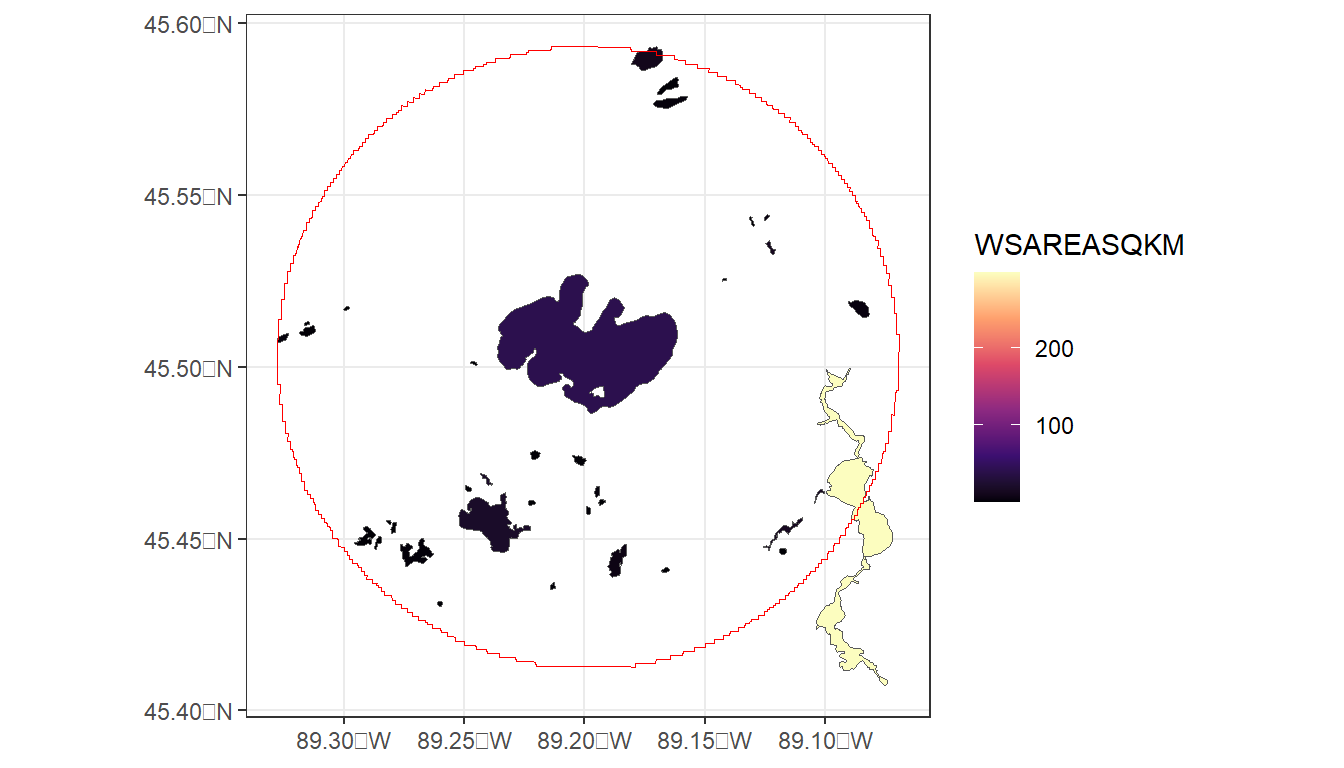
ggplot() +
geom_point(data = pelican_neighbors,
aes(x = WSAREASQKM,
y = areasqkm),
size = 4, alpha = 0.5) +
scale_x_log10() +
xlab('Watershed Area (Km2)') +
scale_y_log10() +
ylab('Lake Area (Km2)') +
theme_bw()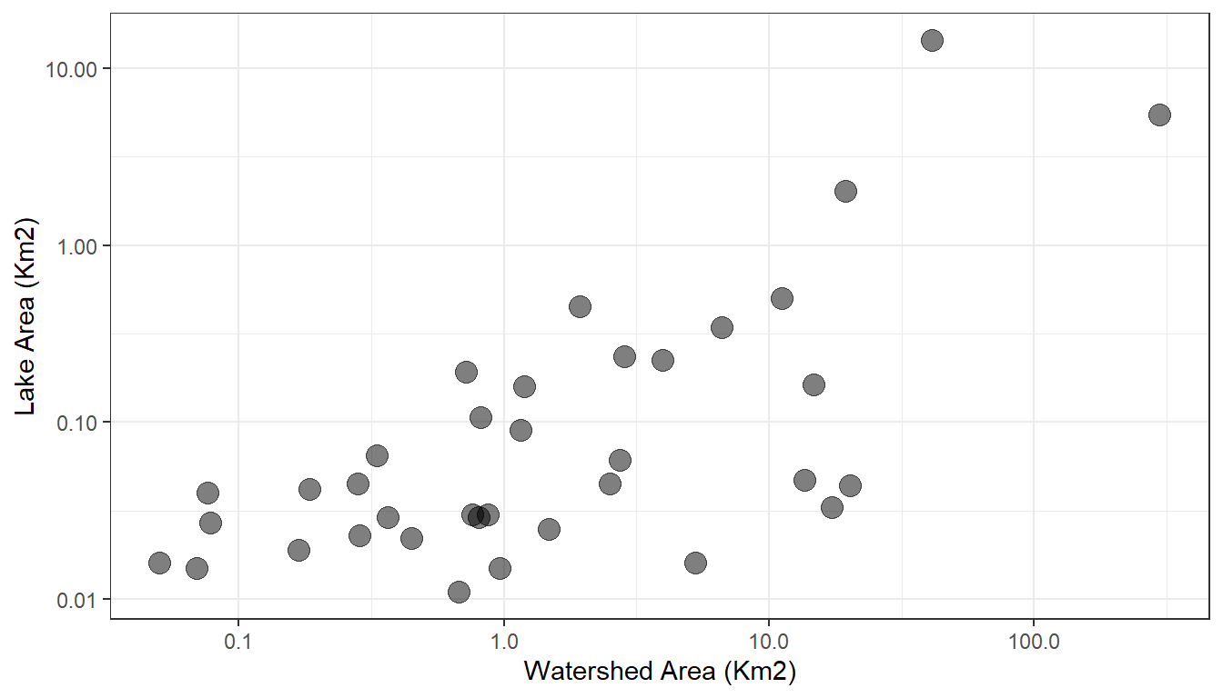
In the next sections, we will put what we have learned about GIS in R together with the spmodel package to model two types of data. In the first example, we will model the specific conductivity of lakes in several midwestern states. Second, we will model the presence/absence of a damselfly genus (Argia) in the northeastern U.S. streams. We’ll access Argia presences/absences via another R package that was recently released called finsyncR. ## R Code Appendix
library(StreamCatTools)
library(tidyverse)
library(sf)
library(terra)
library(FedData)
library(nhdplusTools)
library(mapview)
# Calapooia Watershed
latitude <- 44.62892
longitude <- -123.13113
# Make point sf of sample site
pt <- data.frame(site_name = 'Calapooia',
longitude = longitude,
latitude = latitude) %>%
st_as_sf(coords = c('longitude', 'latitude'), crs = 4269)
# Generate watershed
cal_ws <- pt %>%
nhdplusTools::discover_nhdplus_id() %>%
list(featureSource = "comid", featureID = .) %>%
nhdplusTools::get_nldi_basin() %>%
st_transform(crs = 5070)
# Download NLCD for 2019
nlcd <- get_nlcd(
template = cal_ws,
year = 2019,
label = 'Calapooia') %>%
terra::project('epsg:5070', method = 'near')
# Use terra to extract the watershed metrics
terra::extract(nlcd,
terra::vect(cal_ws)) %>%
group_by(Class) %>%
summarise(count = n()) %>%
mutate(percent = (count / sum(count)) * 100) %>%
filter(Class == 'Cultivated Crops')
comid <- sc_get_comid(pt)
sc_get_data(comid = comid,
metric = 'PctCrop2019',
aoi = 'watershed')
sc_get_data(comid = comid,
metric = 'PctCrop2019',
aoi = 'catchment,watershed')
trib_pt2 <- st_sfc(st_point(c(longitude, latitude)), crs = 4269)
start_comid <- nhdplusTools::discover_nhdplus_id(trib_pt2)
ws_source <- list(featureSource = "comid", featureID = start_comid)

trib_ws2 <- nhdplusTools::get_nldi_basin(nldi_feature = ws_source)

streams <- nhdplusTools::navigate_nldi(ws_source, mode = "UT",
                                       distance_km = 2000) %>%
  pluck('UT_flowlines')

# Use get_nhdplus to access the individual stream sub-catchments
all_catchments <- nhdplusTools::get_nhdplus(comid = streams$nhdplus_comid,
                                            realization = 'catchment')

focal_cat <- nhdplusTools::get_nhdplus(comid = start_comid,
                                       realization = 'catchment')

mapview(streams, color='blue', legend = FALSE) +
  mapview(focal_cat, alpha.regions=.08, col.regions = 'red') +
  mapview(all_catchments, alpha.regions=.08, col.regions = 'yellow')
sc_get_data(comid = comid,
metric = 'PctCrop2019',
aoi = 'catchment,riparian_catchment,watershed,riparian_watershed') %>%
as.data.frame()
iowa_crop <- sc_get_data(state = 'IA',
                         metric = 'PctCrop2019',
                         aoi = 'watershed')

ggplot() +
  geom_histogram(data = iowa_crop,
                 aes(x = PCTCROP2019WS)) +
  theme_bw()
iowa_crop <- sc_get_data(state = 'IA',
                         metric = 'PctCrop2001, PctCrop2019',
                         aoi = 'watershed')

# Pivot table to long format
iowa_crop_long <- iowa_crop %>%
  pivot_longer(
    cols = !COMID:WSAREASQKM,
    values_to = 'PctCrop',
    names_to = 'Year')

ggplot() +
  geom_boxplot(data = iowa_crop_long,
               aes(x = Year,
                   y = PctCrop)) +
  theme_bw()
# Pelican Lake, WI
latitude <- 45.502840
longitude <- -89.198694
pelican_pt <- data.frame(site_name = 'Pelican Lake',
latitude = latitude,
longitude = longitude) %>%
st_as_sf(coords = c('longitude', 'latitude'), crs = 4326)
pelican_lake <- nhdplusTools::get_waterbodies(pelican_pt)
comid <- pelican_lake %>%
pull(comid)
lc_get_data(metric = 'elev, cao, sand, om, pctdecid2019',
aoi = 'watershed',
comid = comid)
# 100km buffer to pelican point
pelican_buffer <-
  pelican_pt %>%
  st_buffer(10000)

pelican_neighbors <- nhdplusTools::get_waterbodies(pelican_buffer) %>%
  filter(ftype == 'LakePond') %>%
  rename(COMID = comid)

comids <- pelican_neighbors %>%
  pull(COMID)

lc_data <- lc_get_data(metric = 'elev, cao, sand, om, pctdecid2019',
                       aoi = 'watershed',
                       comid = comids)

pelican_neighbors <-
  pelican_neighbors %>%
  left_join(lc_data, join_by('COMID'))

ggplot() +
  geom_sf(data = pelican_neighbors,
          aes(fill = WSAREASQKM)) +
  geom_sf(data = pelican_buffer,
          color = 'red',
          fill = NA) +
  scale_fill_viridis_c(option = "magma") +
  theme_bw()
ggplot() +
  geom_point(data = pelican_neighbors,
             aes(x = WSAREASQKM,
                 y = areasqkm),
             size = 4, alpha = 0.5) +
  scale_x_log10() +
  xlab('Watershed Area (Km2)') +
  scale_y_log10() +
  ylab('Lake Area (Km2)') +
  theme_bw()