An Overview of Basic Features in spmodel

Michael Dumelle, Matt Higham, and Jay M. Ver Hoef

Introduction

The spmodel package is used to fit and summarize spatial models and make predictions at unobserved locations (Kriging). This vignette provides an overview of basic features in spmodel. We load spmodel by running

library(spmodel)

If you use spmodel in a formal publication or report, please cite it. Citing spmodel lets us devote more resources to it in the future. We view the spmodel citation by running

citation(package = "spmodel")

#> 
#> To cite spmodel in publications use:
#> 
#>   Dumelle M, Higham M, Ver Hoef JM (2023). spmodel: Spatial statistical
#>   modeling and prediction in R. PLOS ONE 18(3): e0282524.
#>   https://doi.org/10.1371/journal.pone.0282524
#> 
#> A BibTeX entry for LaTeX users is
#> 
#>   @Article{,
#>     title = {{spmodel}: Spatial statistical modeling and prediction in {R}},
#>     author = {Michael Dumelle and Matt Higham and Jay M. {Ver Hoef}},
#>     journal = {PLOS ONE},
#>     year = {2023},
#>     volume = {18},
#>     number = {3},
#>     pages = {1--32},
#>     doi = {10.1371/journal.pone.0282524},
#>     url = {https://doi.org/10.1371/journal.pone.0282524},
#>   }

There are two additional spmodel vignettes:

• A detailed guide to spmodel: vignette("guide", "spmodel")
• Technical details regarding many functions: vignette("technical", "spmodel")

The Data

Many of the data sets we use in this vignette are sf objects. sf objects are data frames (or tibbles) with a special structure that stores spatial information. They are built using the sf (Pebesma 2018) package, which is installed alongside spmodel. We will use six data sets throughout this vignette:

• moss: An sf object with heavy metal concentrations in Alaska.
• sulfate: An sf object with sulfate measurements in the conterminous United States.
• sulfate_preds: An sf object with locations at which to predict sulfate measurements in the conterminous United States.
• caribou: A tibble (a special data.frame) for a caribou foraging experiment in Alaska.
• moose: An sf object with moose measurements in Alaska.
• moose_preds: An sf object with locations at which to predict moose measurements in Alaska.

We will create visualizations using ggplot2 (Wickham 2016), which we load by running

library(ggplot2)

ggplot2 is only installed alongside spmodel when dependencies = TRUE in install.packages(), so check that it is installed before reproducing any visualizations in this vignette.

Spatial Linear Models

Spatial linear models for a quantitative response vector \(\mathbf{y}\) have spatially dependent random errors and are often parameterized as

\[\begin{equation*} \mathbf{y} = \mathbf{X} \boldsymbol{\beta} + \boldsymbol{\tau} + \boldsymbol{\epsilon}, \end{equation*}\]

where \(\mathbf{X}\) is a matrix of explanatory variables (usually including a column of 1’s for an intercept), \(\boldsymbol{\beta}\) is a vector of fixed effects that describe the average impact of \(\mathbf{X}\) on \(\mathbf{y}\), \(\boldsymbol{\tau}\) is a vector of spatially dependent (correlated) random errors, and \(\boldsymbol{\epsilon}\) is a vector of spatially independent (uncorrelated) random errors. The spatial dependence of \(\boldsymbol{\tau}\) is explicitly specified using a spatial covariance function that incorporates the variance of \(\boldsymbol{\tau}\), often called the partial sill, and a range parameter that controls the behavior of the spatial covariance. The variance of \(\boldsymbol{\epsilon}\) is often called the nugget.

Spatial linear models are fit in spmodel for point-referenced and areal data. Data are point-referenced when the elements in \(\mathbf{y}\) are observed at point-locations indexed by x-coordinates and y-coordinates on a spatially continuous surface with an infinite number of locations. The splm() function is used to fit spatial linear models for point-referenced data (these are often called geostatistical models). Data are areal when the elements in \(\mathbf{y}\) are observed as part of a finite network of polygons whose connections are indexed by a neighborhood structure. For example, the polygons may represent counties in a state who are neighbors if they share at least one boundary. The spautor() function is used to fit spatial linear models for areal data (these are often called spatial autoregressive models). This vignette focuses on spatial linear models for point-referenced data, though spmodel’s other vignettes discuss spatial linear models for areal data.

The splm() function has similar syntax and output as the commonly used lm() function used to fit non-spatial linear models. splm() generally requires at least three arguments:

• formula: a formula that describes the relationship between the response variable and explanatory variables.
  • formula uses the same syntax as the formula argument in lm()
• data: a data.frame or sf object that contains the response variable, explanatory variables, and spatial information.
• spcov_type: the spatial covariance type ("exponential", "spherical", "matern", etc).

If data is an sf object, the coordinate information is taken from the object’s geometry. If data is a data.frame (or tibble), then xcoord and ycoord are required arguments to splm() that specify the columns in data representing the x-coordinates and y-coordinates, respectively. spmodel uses the spatial coordinates “as-is,” meaning that spmodel does not perform any projections. To project your data or change the coordinate reference system, use sf::st_transform(). If an sf object with polygon geometries is given to splm(), the centroids of each polygon are used to fit the spatial linear model.

Next we show the basic features and syntax of splm() using the Alaskan moss data. We study the impact of log distance to the road (log_dist2road) on log zinc concentration (log_Zn). We view the first few rows of the moss data by running

moss

#> Simple feature collection with 365 features and 7 fields
#> Geometry type: POINT
#> Dimension:     XY
#> Bounding box:  xmin: -445884.1 ymin: 1929616 xmax: -383656.8 ymax: 2061414
#> Projected CRS: NAD83 / Alaska Albers
#> # A tibble: 365 x 8
#>    sample field_dup lab_rep year  sideroad log_dist2road log_Zn
#>    <fct>  <fct>     <fct>   <fct> <fct>            <dbl>  <dbl>
#>  1 001PR  1         1       2001  N                 2.68   7.33
#>  2 001PR  1         2       2001  N                 2.68   7.38
#>  3 002PR  1         1       2001  N                 2.54   7.58
#>  4 003PR  1         1       2001  N                 2.97   7.63
#>  5 004PR  1         1       2001  N                 2.72   7.26
#>  6 005PR  1         1       2001  N                 2.76   7.65
#>  7 006PR  1         1       2001  S                 2.30   7.59
#>  8 007PR  1         1       2001  N                 2.78   7.16
#>  9 008PR  1         1       2001  N                 2.93   7.19
#> 10 009PR  1         1       2001  N                 2.79   8.07
#> # ... with 355 more rows, and 1 more variable: geometry <POINT [m]>

We can visualize the distribution of log zinc concentration (log_Zn) by running

ggplot(moss, aes(color = log_Zn)) +
  geom_sf() +
  scale_color_viridis_c()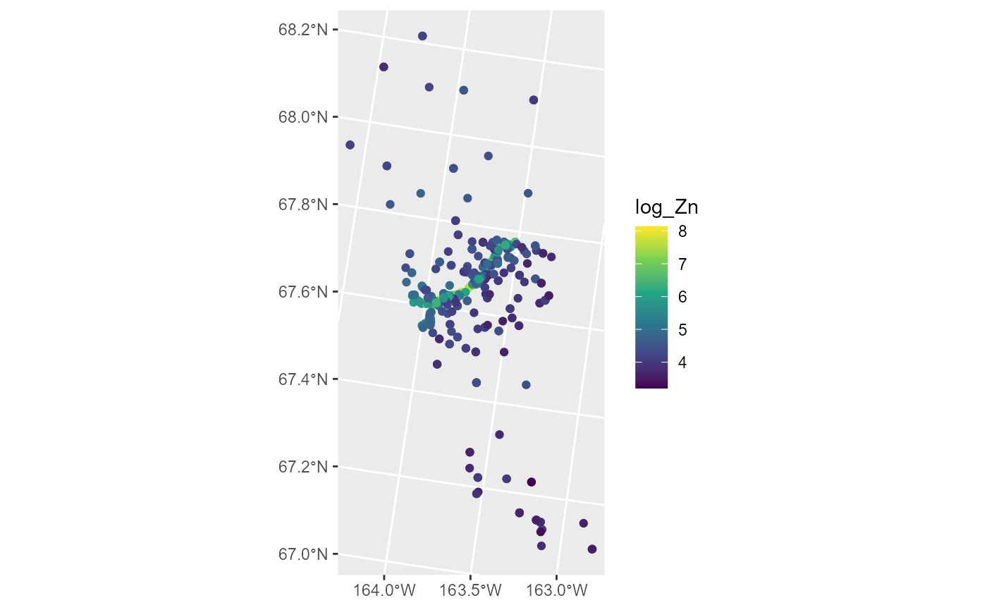

Log zinc concentration appears highest in the middle of the spatial domain, which has a road running through it. We fit a spatial linear model regressing log zinc concentration on log distance to the road using an exponential spatial covariance function by running

spmod <- splm(log_Zn ~ log_dist2road, data = moss, spcov_type = "exponential")

The estimation method is specified via the estmethod argument, which has a default value of "reml" for restricted maximum likelihood. Other estimation methods are "ml" for maximum likelihood, "sv-wls" for semivariogram weighted least squares, and "sv-cl" for semivariogram composite likelihood.

Printing spmod shows the function call, the estimated fixed effect coefficients, and the estimated spatial covariance parameters. de is the estimated variance of \(\boldsymbol{\tau}\) (the spatially dependent random error), ie is the estimated variance of \(\boldsymbol{\epsilon}\) (the spatially independent random error), and range is the range parameter.

print(spmod)

#> 
#> Call:
#> splm(formula = log_Zn ~ log_dist2road, data = moss, spcov_type = "exponential")
#> 
#> 
#> Coefficients (fixed):
#>   (Intercept)  log_dist2road  
#>        9.7683        -0.5629  
#> 
#> 
#> Coefficients (exponential spatial covariance):
#>        de         ie      range  
#> 3.595e-01  7.897e-02  8.237e+03

Next we show how to obtain more detailed summary information from the fitted model.

Model Summaries

We summarize the fitted model by running

summary(spmod)

#> 
#> Call:
#> splm(formula = log_Zn ~ log_dist2road, data = moss, spcov_type = "exponential")
#> 
#> Residuals:
#>     Min      1Q  Median      3Q     Max 
#> -2.6801 -1.3606 -0.8103 -0.2485  1.1298 
#> 
#> Coefficients (fixed):
#>               Estimate Std. Error z value Pr(>|z|)    
#> (Intercept)    9.76825    0.25216   38.74   <2e-16 ***
#> log_dist2road -0.56287    0.02013  -27.96   <2e-16 ***
#> ---
#> Signif. codes:  0 '***' 0.001 '**' 0.01 '*' 0.05 '.' 0.1 ' ' 1
#> 
#> Pseudo R-squared: 0.683
#> 
#> Coefficients (exponential spatial covariance):
#>        de        ie     range 
#> 3.595e-01 7.897e-02 8.237e+03

Similar to summaries of lm() objects, summaries of splm() objects include the original function call, residuals, and a coefficients table of fixed effects. Log zinc concentration appears to significantly decrease with log distance from the road, as evidenced by the small p-value associated with the asymptotic z-test. A pseudo r-squared is also returned, which quantifies the proportion of variability explained by the fixed effects.

In the remainder of this subsection, we describe the broom (Robinson, Hayes, and Couch 2021) functions tidy(), glance() and augment(). tidy() tidies coefficient output in a convenient tibble, glance() glances at model-fit statistics, and augment() augments the data with fitted model diagnostics.

We tidy the fixed effects by running

tidy(spmod)

#> # A tibble: 2 x 5
#>   term          estimate std.error statistic p.value
#>   <chr>            <dbl>     <dbl>     <dbl>   <dbl>
#> 1 (Intercept)      9.77     0.252       38.7       0
#> 2 log_dist2road   -0.563    0.0201     -28.0       0

We glance at the model-fit statistics by running

glance(spmod)

#> # A tibble: 1 x 9
#>       n     p  npar value   AIC  AICc logLik deviance pseudo.r.squared
#>   <int> <dbl> <int> <dbl> <dbl> <dbl>  <dbl>    <dbl>            <dbl>
#> 1   365     2     3  367.  373.  373.  -184.     363.            0.683

The columns of this tibble represent:

• n: The sample size
• p: The number of fixed effects (linearly independent columns in \(\mathbf{X}\))
• npar: The number of estimated covariance parameters
• value: The value of the minimized objective function used when fitting the model
• AIC: The Akaike Information Criterion (AIC)
• AICc: The AIC with a small sample size correction
• logLik: The log-likelihood
• deviance: The deviance
• pseudo.r.squared: The pseudo r-squared

The glances() function can be used to glance at multiple models at once. Suppose we wanted to compare the current model, which uses an exponential spatial covariance, to a new model without spatial covariance (equivalent to a model fit using lm()). We do this using glances() by running

lmod <- splm(log_Zn ~ log_dist2road, data = moss, spcov_type = "none")
glances(spmod, lmod)

#> # A tibble: 2 x 10
#>   model     n     p  npar value   AIC  AICc logLik deviance pseudo.r.squared
#>   <chr> <int> <dbl> <int> <dbl> <dbl> <dbl>  <dbl>    <dbl>            <dbl>
#> 1 spmod   365     2     3  367.  373.  373.  -184.     363.            0.683
#> 2 lmod    365     2     1  634.  636.  636.  -317.     363.            0.671

The much lower AIC and AICc for the spatial linear model indicates it is a much better fit to the data. Outside of glance() and glances(), the functions AIC(), AICc(), logLik(), deviance(), and pseudoR2() are available to compute the relevant statistics.

We augment the data with diagnostics by running

augment(spmod)

#> Simple feature collection with 365 features and 7 fields
#> Geometry type: POINT
#> Dimension:     XY
#> Bounding box:  xmin: -445884.1 ymin: 1929616 xmax: -383656.8 ymax: 2061414
#> Projected CRS: NAD83 / Alaska Albers
#> # A tibble: 365 x 8
#>    log_Zn log_dist2road .fitted .resid   .hat .cooksd .std.resid
#>  *  <dbl>         <dbl>   <dbl>  <dbl>  <dbl>   <dbl>      <dbl>
#>  1   7.33          2.68    8.26 -0.928 0.0200 0.0142       1.18 
#>  2   7.38          2.68    8.26 -0.880 0.0200 0.0186       1.35 
#>  3   7.58          2.54    8.34 -0.755 0.0225 0.00482      0.647
#>  4   7.63          2.97    8.09 -0.464 0.0197 0.0305       1.74 
#>  5   7.26          2.72    8.24 -0.977 0.0215 0.131        3.45 
#>  6   7.65          2.76    8.21 -0.568 0.0284 0.0521       1.89 
#>  7   7.59          2.30    8.47 -0.886 0.0300 0.0591       1.96 
#>  8   7.16          2.78    8.20 -1.05  0.0335 0.00334      0.439
#>  9   7.19          2.93    8.12 -0.926 0.0378 0.0309       1.26 
#> 10   8.07          2.79    8.20 -0.123 0.0314 0.00847      0.723
#> # ... with 355 more rows, and 1 more variable: geometry <POINT [m]>

The columns of this tibble represent:

• log_Zn: The log zinc concentration.
• log_dist2road: The log distance to the road.
• .fitted: The fitted values (the estimated mean given the explanatory variable values).
• .resid: The residuals (the response minus the fitted values).
• .hat: The leverage (hat) values.
• .cooksd: The Cook’s distance
• .std.residuals: Standardized residuals
• geometry: The spatial information in the sf object.

By default, augment() only returns the variables in the data used by the model. All variables from the original data are returned by setting drop = FALSE. Many of these model diagnostics can be visualized by running plot(spmod). We can learn more about plot() in spmodel by running help("plot.spmodel", "spmodel").

Prediction (Kriging)

Commonly a goal of a data analysis is to make predictions at unobserved locations. In spatial contexts, prediction is often called Kriging. Next we use the sulfate data to build a spatial linear model of sulfate measurements in the conterminous United States with the goal of making sulfate predictions (Kriging) for the unobserved locations in sulfate_preds.

We visualize the distribution of sulfate by running

ggplot(sulfate, aes(color = sulfate)) +
  geom_sf(size = 2) +
  scale_color_viridis_c(limits = c(0, 45))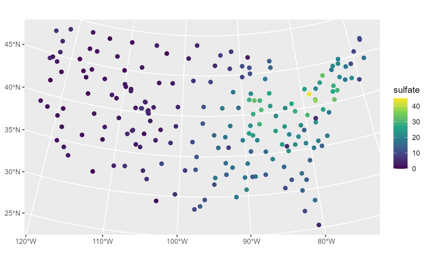

Sulfate appears spatially dependent, as measurements are highest in the Northeast and lowest in the Midwest and West.

We fit a spatial linear model regressing sulfate on an intercept using a spherical spatial covariance function by running

sulfmod <- splm(sulfate ~ 1, data = sulfate, spcov_type =  "spherical")

We make predictions at the locations in sulfate_preds and store them as a new variable called preds in the sulfate_preds data set by running

sulfate_preds$preds <- predict(sulfmod, newdata = sulfate_preds)

We visualize these predictions by running

ggplot(sulfate_preds, aes(color = preds)) +
  geom_sf(size = 2) +
  scale_color_viridis_c(limits = c(0, 45))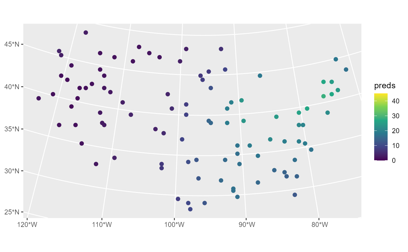

These predictions have similar sulfate patterns as in the observed data (predicted values are highest in the Northeast and lowest in the Midwest and West). Next we remove the model predictions from sulfate_preds before showing how augment() can be used to obtain the same predictions:

sulfate_preds$preds <- NULL

While augment() was previously used to augment the original data with model diagnostics, it can also be used to augment the newdata data with predictions:

augment(sulfmod, newdata = sulfate_preds)

#> Simple feature collection with 100 features and 1 field
#> Geometry type: POINT
#> Dimension:     XY
#> Bounding box:  xmin: -2283774 ymin: 582930.5 xmax: 1985906 ymax: 3037173
#> Projected CRS: NAD83 / Conus Albers
#> # A tibble: 100 x 2
#>    .fitted            geometry
#>  *   <dbl>         <POINT [m]>
#>  1    1.40  (-1771413 1752976)
#>  2   24.5    (1018112 1867127)
#>  3    8.99 (-291256.8 1553212)
#>  4   16.4    (1274293 1267835)
#>  5    4.91 (-547437.6 1638825)
#>  6   26.7    (1445080 1981278)
#>  7    3.00  (-1629090 3037173)
#>  8   14.3    (1302757 1039534)
#>  9    1.49  (-1429838 2523494)
#> 10   14.4    (1131970 1096609)
#> # ... with 90 more rows

Here .fitted represents the predictions.

Confidence intervals for the mean response or prediction intervals for the predicted response can be obtained by specifying the interval argument in predict() and augment():

augment(sulfmod, newdata = sulfate_preds, interval = "prediction")

#> Simple feature collection with 100 features and 3 fields
#> Geometry type: POINT
#> Dimension:     XY
#> Bounding box:  xmin: -2283774 ymin: 582930.5 xmax: 1985906 ymax: 3037173
#> Projected CRS: NAD83 / Conus Albers
#> # A tibble: 100 x 4
#>    .fitted .lower .upper            geometry
#>  *   <dbl>  <dbl>  <dbl>         <POINT [m]>
#>  1    1.40  -6.62   9.42  (-1771413 1752976)
#>  2   24.5   17.0   32.0    (1018112 1867127)
#>  3    8.99   1.09  16.9  (-291256.8 1553212)
#>  4   16.4    8.67  24.2    (1274293 1267835)
#>  5    4.91  -2.80  12.6  (-547437.6 1638825)
#>  6   26.7   19.2   34.2    (1445080 1981278)
#>  7    3.00  -4.92  10.9   (-1629090 3037173)
#>  8   14.3    6.76  21.8    (1302757 1039534)
#>  9    1.49  -6.34   9.32  (-1429838 2523494)
#> 10   14.4    6.74  22.1    (1131970 1096609)
#> # ... with 90 more rows

By default, predict() and augment() compute 95% intervals, though this can be changed using the level argument.

While the fitted model in this example only used an intercept, the same code is used for prediction with fitted models having explanatory variables. If explanatory variables were used to fit the model, the same explanatory variables must be included in newdata with the same names they have in data. If data is a data.frame, coordinates must be included in newdata with the same names as they have in data. If data is an sf object, coordinates must be included in newdata with the same geometry name as they have in data. When using projected coordinates, the projection for newdata should be the same as the projection for data.

An Additional Example

We now use the caribou data from a foraging experiment conducted in Alaska to show an application of splm() to data stored in a tibble (data.frame) instead of an sf object. In caribou, the x-coordinates are stored in the x column and the y-coordinates are stored in the y column. We view the first few rows of caribou by running

caribou

#> # A tibble: 30 x 5
#>    water tarp      z     x     y
#>    <fct> <fct> <dbl> <dbl> <dbl>
#>  1 Y     clear  2.42     1     6
#>  2 Y     shade  2.44     2     6
#>  3 Y     none   1.81     3     6
#>  4 N     clear  1.97     4     6
#>  5 N     shade  2.38     5     6
#>  6 Y     none   2.22     1     5
#>  7 N     clear  2.10     2     5
#>  8 Y     clear  1.80     3     5
#>  9 Y     shade  1.96     4     5
#> 10 Y     none   2.10     5     5
#> # ... with 20 more rows

We fit a spatial linear model regressing nitrogen percentage (z) on water presence (water) and tarp cover (tarp) by running

cariboumod <- splm(z ~ water + tarp, data = caribou,
                   spcov_type = "exponential", xcoord = x, ycoord = y)

An analysis of variance can be conducted to assess the overall impact of the tarp variable, which has three levels (clear, shade, and none), and the water variable, which has two levels (water and no water). We perform an analysis of variance by running

anova(cariboumod)

#> Analysis of Variance Table
#> 
#> Response: z
#>             Df    Chi2 Pr(>Chi2)    
#> (Intercept)  1 43.4600 4.327e-11 ***
#> water        1  1.6603 0.1975631    
#> tarp         2 15.4071 0.0004512 ***
#> ---
#> Signif. codes:  0 '***' 0.001 '**' 0.01 '*' 0.05 '.' 0.1 ' ' 1

There seems to be significant evidence that at least one tarp cover impacts nitrogen. Note that, like in summary(), these p-values are associated with an asymptotic hypothesis test (here, an asymptotic Chi-squared test).

Spatial Generalized Linear Models

When building spatial linear models, the response vector \(\mathbf{y}\) is typically assumed Gaussian (given \(\mathbf{X}\)). Relaxing this assumption on the distribution of \(\mathbf{y}\) yields a rich class of spatial generalized linear models that can describe binary data, proportion data, count data, and skewed data. Spatial generalized linear models are parameterized as \[\begin{equation*} g(\boldsymbol{\mu}) = \boldsymbol{\eta} = \mathbf{X} \boldsymbol{\beta} + \boldsymbol{\tau} + \boldsymbol{\epsilon}, \end{equation*}\] where \(g(\cdot)\) is called a link function, \(\boldsymbol{\mu}\) is the mean of \(\mathbf{y}\), and the remaining terms \(\mathbf{X}\), \(\boldsymbol{\beta}\), \(\boldsymbol{\tau}\), \(\boldsymbol{\epsilon}\) represent the same quantities as for the spatial linear models (Section\(~\)). The link function, \(g(\cdot)\), “links” a function of \(\boldsymbol{\mu}\) to the linear term \(\boldsymbol{\eta}\), denoted here as \(\mathbf{X} \boldsymbol{\beta} + \boldsymbol{\tau} + \boldsymbol{\epsilon}\), which is familiar from spatial linear models. Note that the linking of \(\boldsymbol{\mu}\) to \(\boldsymbol{\eta}\) applies element-wise to each vector. Each link function \(g(\cdot)\) has a corresponding inverse link function, \(g^{-1}(\cdot)\). The inverse link function “links” a function of \(\boldsymbol{\eta}\) to \(\boldsymbol{\mu}\). Notice that for spatial generalized linear models, we are not modeling \(\mathbf{y}\) directly as we do for spatial linear models, but rather we are modeling a function of the mean of \(\mathbf{y}\). Also notice that \(\boldsymbol{\eta}\) is unconstrained but \(\boldsymbol{\mu}\) is usually constrained in some way (e.g., positive). Next we discuss the specific distributions and link functions used in spmodel.

spmodel allows fitting of spatial generalized linear models when \(\mathbf{y}\) is a binomial (or Bernoulli), beta, Poisson, negative binomial, gamma, or inverse Gaussian random vector. For binomial and beta \(\mathbf{y}\), the logit link function is defined as \(g(\boldsymbol{\mu}) = \ln(\frac{\boldsymbol{\mu}}{1 - \boldsymbol{\mu}}) = \boldsymbol{\eta}\), and the inverse logit link function is defined as \(g^{-1}(\boldsymbol{\eta}) = \frac{\exp(\boldsymbol{\eta})}{1 + \exp(\boldsymbol{\eta})} = \boldsymbol{\mu}\). For Poisson, negative binomial, gamma, and inverse Gaussian \(\mathbf{y}\), the log link function is defined as \(g(\boldsymbol{\mu}) = \ln(\boldsymbol{\mu}) = \boldsymbol{\eta}\), and the inverse log link function is defined as \(g^{-1}(\boldsymbol{\eta}) = \exp(\boldsymbol{\eta}) = \boldsymbol{\mu}\).

As with spatial linear models, spatial generalized linear models are fit in spmodel for point-referenced and areal data. The spglm() function is used to fit spatial generalized linear models for point-referenced data, and the spgautor() function is used to fit spatial generalized linear models for areal data. Though this vignette focuses on point-referenced data, spmodel’s other vignettes discuss spatial generalized linear models for areal data.

The spglm() function is quite similar to the splm() function, though one additional argument is required:

• family: the generalized linear model family (i.e., the distribution of \(\mathbf{y}\)). family can be binomial, beta, poisson, nbinomial, Gamma, or inverse.gaussian.
  • family uses similar syntax as the family argument in glm().
  • One difference between family in spglm() compared to family in glm() is that the link function is fixed in spglm().

Next we show the basic features and syntax of spglm() using the moose data. We study the impact of elevation (elev) on the presence of moose (presence) observed at a site location in Alaska. presence equals one if at least one moose was observed at the site and zero otherwise. We view the first few rows of the moose data by running

moose

#> Simple feature collection with 218 features and 4 fields
#> Geometry type: POINT
#> Dimension:     XY
#> Bounding box:  xmin: 269085 ymin: 1416151 xmax: 419976.2 ymax: 1541763
#> Projected CRS: NAD83 / Alaska Albers
#> First 10 features:
#>        elev strat count presence                 geometry
#> 1  468.9167     L     0        0 POINT (293542.6 1541016)
#> 2  362.3125     L     0        0 POINT (298313.1 1533972)
#> 3  172.7500     M     0        0 POINT (281896.4 1532516)
#> 4  279.6250     L     0        0 POINT (298651.3 1530264)
#> 5  619.6000     L     0        0 POINT (311325.3 1527705)
#> 6  164.1250     M     0        0 POINT (291421.5 1518398)
#> 7  163.5000     M     0        0 POINT (287298.3 1518035)
#> 8  186.3500     L     0        0 POINT (279050.9 1517324)
#> 9  362.3125     L     0        0 POINT (346145.9 1512479)
#> 10 430.5000     L     0        0 POINT (321354.6 1509966)

We can visualize the distribution of moose presence by running

ggplot(moose, aes(color = presence)) +
  scale_color_viridis_d() +
  geom_sf(size = 2)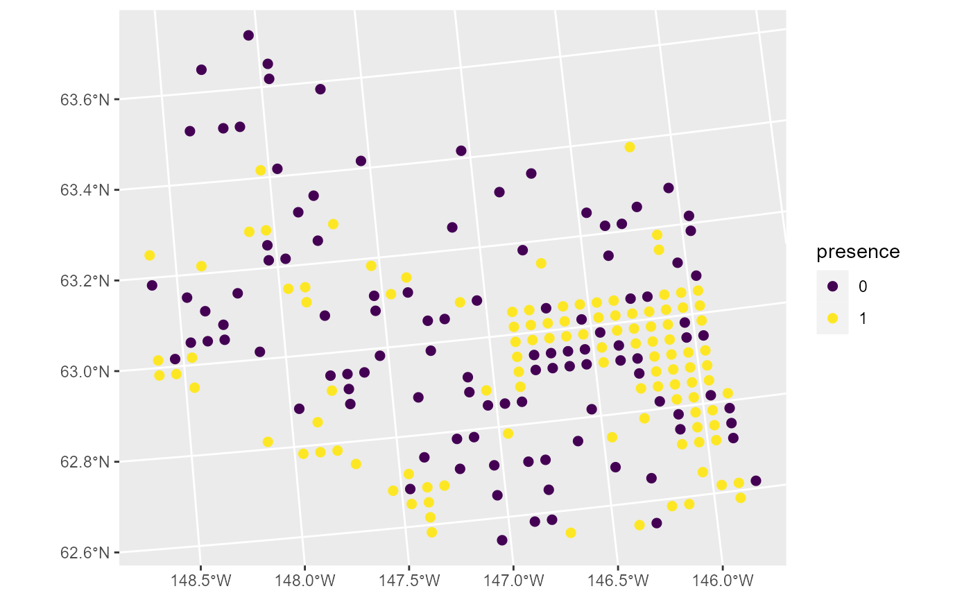 

One example of a generalized linear model is a binomial (e.g., logistic) regression model. Binomial regression models are often used to model presence data such as this. To quantify the relationship between moose presence and elevation, we fit a spatial binomial regression model (a specific spatial generalized linear model) by running

binmod <- spglm(presence ~ elev, family = "binomial",
                data  = moose, spcov_type = "exponential")

The estimation method is specified via the estmethod argument, which has a default value of "reml" for restricted maximum likelihood. The other estimation method is "ml" for maximum likelihood.

Printing binmod shows the function call, the estimated fixed effect coefficients (on the link scale), the estimated spatial covariance parameters, and a dispersion parameter. The dispersion parameter is estimated for some spatial generalized linear models and changes the mean-variance relationship of \(\mathbf{y}\). For binomial regression models, the dispersion parameter is not estimated and is always fixed at one.

print(binmod)

#> 
#> Call:
#> spglm(formula = presence ~ elev, family = "binomial", data = moose, 
#>     spcov_type = "exponential")
#> 
#> 
#> Coefficients (fixed):
#> (Intercept)         elev  
#>   -0.874038     0.002365  
#> 
#> 
#> Coefficients (exponential spatial covariance):
#>        de         ie      range  
#> 3.746e+00  4.392e-03  3.203e+04  
#> 
#> 
#> Coefficients (Dispersion for binomial family):
#> dispersion  
#>          1

Model Summaries

We summarize the fitted model by running

summary(binmod)

#> 
#> Call:
#> spglm(formula = presence ~ elev, family = "binomial", data = moose, 
#>     spcov_type = "exponential")
#> 
#> Deviance Residuals:
#>     Min      1Q  Median      3Q     Max 
#> -1.5249 -0.8114  0.5600  0.8306  1.5757 
#> 
#> Coefficients (fixed):
#>              Estimate Std. Error z value Pr(>|z|)
#> (Intercept) -0.874038   1.140953  -0.766    0.444
#> elev         0.002365   0.003184   0.743    0.458
#> 
#> Pseudo R-squared: 0.00311
#> 
#> Coefficients (exponential spatial covariance):
#>        de        ie     range 
#> 3.746e+00 4.392e-03 3.203e+04 
#> 
#> Coefficients (Dispersion for binomial family):
#> dispersion 
#>          1

Similar to summaries of glm() objects, summaries of spglm() objects include the original function call, summary statistics of the deviance residuals, and a coefficients table of fixed effects. The logit of moose presence probability does not appear to be related to elevation, as evidenced by the large p-value associated with the asymptotic z-test. A pseudo r-squared is also returned, which quantifies the proportion of variability explained by the fixed effects. The spatial covariance parameters and dispersion parameter are also returned.

The tidy(), glance(), and augment() functions behave similarly for spglm() objects as they do for splm() objects. We tidy the fixed effects (on the link scale) by running

tidy(binmod)

#> # A tibble: 2 x 5
#>   term        estimate std.error statistic p.value
#>   <chr>          <dbl>     <dbl>     <dbl>   <dbl>
#> 1 (Intercept) -0.874     1.14       -0.766   0.444
#> 2 elev         0.00237   0.00318     0.743   0.458

We glance at the model-fit statistics by running

glance(binmod)

#> # A tibble: 1 x 9
#>       n     p  npar value   AIC  AICc logLik deviance pseudo.r.squared
#>   <int> <dbl> <int> <dbl> <dbl> <dbl>  <dbl>    <dbl>            <dbl>
#> 1   218     2     3  692.  698.  698.  -346.     190.          0.00311

We glance at the spatial binomial regression model and a non-spatial binomial regression model by running

glmod <- spglm(presence ~ elev, family = "binomial", data = moose, spcov_type = "none")
glances(binmod, glmod)

#> # A tibble: 2 x 10
#>   model      n     p  npar value   AIC  AICc logLik deviance pseudo.r.squared
#>   <chr>  <int> <dbl> <int> <dbl> <dbl> <dbl>  <dbl>    <dbl>            <dbl>
#> 1 binmod   218     2     3  692.  698.  698.  -346.     190.          0.00311
#> 2 glmod    218     2     1  715.  717.  717.  -358.     302.          0.00185

The lower AIC and AICc for the spatial binomial regression model indicates it is a much better fit to the data.

We augment the data with diagnostics by running

augment(binmod)

#> Simple feature collection with 218 features and 7 fields
#> Geometry type: POINT
#> Dimension:     XY
#> Bounding box:  xmin: 269085 ymin: 1416151 xmax: 419057.4 ymax: 1541016
#> Projected CRS: NAD83 / Alaska Albers
#> # A tibble: 218 x 8
#>    presence  elev .fitted .resid    .hat  .cooksd .std.resid
#>  * <fct>    <dbl>   <dbl>  <dbl>   <dbl>    <dbl>      <dbl>
#>  1 0         469.  0.150  -0.571 0.0500  0.00904      -0.586
#>  2 0         362.  0.107  -0.477 0.0168  0.00198      -0.481
#>  3 0         173.  0.104  -0.468 0.00213 0.000235     -0.469
#>  4 0         280.  0.0939 -0.444 0.00616 0.000615     -0.445
#>  5 0         620.  0.198  -0.664 0.136   0.0402       -0.714
#>  6 0         164.  0.130  -0.528 0.00260 0.000364     -0.528
#>  7 0         164.  0.135  -0.538 0.00269 0.000392     -0.539
#>  8 0         186.  0.166  -0.603 0.00332 0.000607     -0.604
#>  9 0         362.  0.168  -0.606 0.0245  0.00474      -0.614
#> 10 0         430.  0.225  -0.714 0.0528  0.0150       -0.734
#> # ... with 208 more rows, and 1 more variable: geometry <POINT [m]>

Prediction (Kriging)

For spatial generalized linear models, we are predicting the mean of the process generating the observation rather than the observation itself. We make predictions of moose presence probability at the locations in moose_preds by running

moose_preds$preds <- predict(binmod, newdata = moose_preds, type = "response")

The type argument specifies whether predictions are returned on the link or response (inverse link) scale. We visualize these predictions by running

ggplot(moose_preds, aes(color = preds)) + 
  geom_sf(size = 2) +
  scale_color_viridis_c(limits = c(0, 1))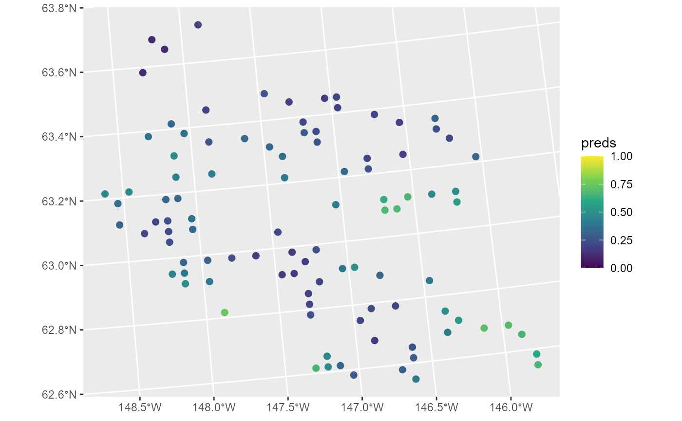

These predictions have similar spatial patterns as moose presence the observed data. Next we remove the model predictions from moose_preds and show how augment() can be used to obtain the same predictions alongside prediction intervals (on the response scale):

moose_preds$preds <- NULL
augment(binmod, newdata = moose_preds, type = "response", interval = "prediction")

#> Simple feature collection with 100 features and 5 fields
#> Geometry type: POINT
#> Dimension:     XY
#> Bounding box:  xmin: 269386.2 ymin: 1418453 xmax: 419976.2 ymax: 1541763
#> Projected CRS: NAD83 / Alaska Albers
#> # A tibble: 100 x 6
#>     elev strat .fitted .lower .upper           geometry
#>  * <dbl> <chr>   <dbl>  <dbl>  <dbl>        <POINT [m]>
#>  1  143. L       0.705 0.248   0.946 (401239.6 1436192)
#>  2  324. L       0.336 0.0373  0.868 (352640.6 1490695)
#>  3  158. L       0.263 0.0321  0.792 (360954.9 1491590)
#>  4  221. M       0.243 0.0360  0.734 (291839.8 1466091)
#>  5  209. M       0.742 0.270   0.957 (310991.9 1441630)
#>  6  218. L       0.191 0.0196  0.736 (304473.8 1512103)
#>  7  127. L       0.179 0.0226  0.673 (339011.1 1459318)
#>  8  122. L       0.241 0.0344  0.738 (342827.3 1463452)
#>  9  191  L       0.386 0.0414  0.902 (284453.8 1502837)
#> 10  105. L       0.494 0.114   0.882 (391343.9 1483791)
#> # ... with 90 more rows

Function Glossary

Here we list some commonly used spmodel functions.

• AIC(): Compute the AIC.
• AICc(): Compute the AICc.
• anova(): Perform an analysis of variance.
• augment(): Augment data with diagnostics or new data with predictions.
• coef(): Return coefficients.
• confint(): Compute confidence intervals.
• cooks.distance(): Compute Cook’s distance.
• covmatrix(): Return covariance matrices.
• deviance(): Compute the deviance.
• esv(): Compute an empirical semivariogram.
• fitted(): Compute fitted values.
• glance(): Glance at a fitted model.
• glances(): Glance at multiple fitted models.
• hatvalues(): Compute leverage (hat) values.
• logLik(): Compute the log-likelihood.
• loocv(): Perform leave-one-out cross validation.
• model.matrix(): Return the model matrix (\(\mathbf{X}\)).
• plot(): Create fitted model plots.
• predict(): Compute predictions and prediction intervals.
• pseudoR2(): Compute the pseudo r-squared.
• residuals(): Compute residuals.
• spautor(): Fit a spatial linear model for areal data (i.e., spatial autoregressive model).
• spautorRF(): Fit a random forest spatial residual model for areal data.
• spgautor(): Fit a spatial generalized linear model for areal data (i.e., spatial generalized autoregressive model).
• splm(): Fit a spatial linear model for point-referenced data (i.e., geostatistical model).
• splmRF(): Fit a random forest spatial residual model for point-referenced data.
• spglm(): Fit a spatial generalized linear model for point-referenced data (i.e., generalized geostatistical model).
• sprbeta(): Simulate spatially correlated beta random variables.
• sprbinom(): Simulate spatially correlated binomial (Bernoulli) random variables.
• sprgamma(): Simulate spatially correlated gamma random variables.
• sprinvgauss(): Simulate spatially correlated inverse Gaussian random variables.
• sprnbinom(): Simulate spatially correlated negative binomial random variables.
• sprnorm(): Simulate spatially correlated normal (Gaussian) random variables.
• sprpois(): Simulate spatially correlated Poisson random variables.
• summary(): Summarize fitted models.
• tidy(): Tidy fitted models.
• varcomp(): Compare variance components.
• vcov(): Compute variance-covariance matrices of estimated parameters.

For a full list of spmodel functions alongside their documentation, see the documentation manual. Documentation for methods of generic functions that are defined outside of spmodel can be found by running help("generic.spmodel", "spmodel") (e.g., help("summary.spmodel", "spmodel"), help("predict.spmodel", "spmodel"), etc.). Note that ?generic.spmodel is shorthand for help("generic.spmodel", "spmodel").

References

Pebesma, Edzer. 2018. “Simple Features for R: Standardized Support for Spatial Vector Data.” The R Journal 10 (1): 439–46. https://doi.org/10.32614/RJ-2018-009.

Robinson, David, Alex Hayes, and Simon Couch. 2021. Broom: Convert Statistical Objects into Tidy Tibbles. https://CRAN.R-project.org/package=broom.

Wickham, Hadley. 2016. Ggplot2: Elegant Graphics for Data Analysis. Springer-Verlag New York. https://ggplot2.tidyverse.org.