TADA Module 2: Geospatial Functions
TADA Team
2026-07-08
Source:vignettes/TADAModule2.Rmd
TADAModule2.RmdOverview and Setup
Welcome!
Thank you for your interest in Tools for Automated Data Analysis (TADA). TADA is an open-source tool set built in the R programming language. This RMarkdown document walks users through how to download the TADA R package from GitHub, access and parameterize several important functions, and create basic visualizations with a sample data set.
Note: TADA is still under development. New functionality is added weekly, and sometimes we need to make bug fixes in response to tester and user feedback. We appreciate your feedback, patience, and interest in these helpful tools.
If you are interested in contributing to TADA development, more information is available at:
We welcome collaboration with external partners.
Geospatial Functions in TADA
This example Module 2 workflow focuses on the following tasks:
Creating a ML/AU Crosswalk: Use
TADA_CreateAUMLCrosswalkto establish a crosswalk between ATTAINS assessment units and WQP monitoring locations.Map Review: Utilize
TADA_ViewATTAINSto review assessment units and monitoring locations on a map, ensuring accuracy and completeness.Submitting the Crosswalk: Employ
TADA_UpdateATTAINSAUMLCrosswalkto submit an up-to-date assessment unit/WQP monitoring location crosswalk to ATTAINS.Assigning Uses: Use
TADA_AssignUsesToAUto assign specific uses to the assessment units.
A Note About ATTAINS:
The Assessment, Total Maximum Daily Load (TMDL) Tracking and Implementation System (ATTAINS) is an online platform that organizes and combines each state and participating tribe’s Clean Water Act reporting data into a single data repository. The geospatial component of ATTAINS includes spatial representations of each entity’s surface water assessment units as well as their assigned designated uses, their most recent EPA reporting category (i.e., their impairment status), their impaired designated uses, and the parameter(s) causing the impairment.
Within an assessment unit, the criteria or thresholds used to assess water quality typically remain the same and all water features are assessed as one entity (although there are some exceptions, for example if a single assessment unit crosses multiple ecoregions). Depending on the state or tribe, these assessment units can be a specific point or series of points along a waterbody such as a river or lake, a river reach (line), an entire waterbody such as a river or lake (polygon), or even an entire watershed. In other words, assessment units can take the form of point, line, and area (polygon) features, or some combination of all of them. Moreover, it is possible that some assessment units are not geospatially referenced at all, meaning they are not captured in the ATTAINS geospatial database.
Install and Load the EPATADA R Package
First, install and load the remotes package specifying the repo. This is needed before installing EPATADA because it is only available on GitHub (not CRAN).
install.packages("remotes")
# Load the remotes library
library(remotes)
Next, install and load TADA using the remotes package. TADA R Package dependencies will also be downloaded automatically from CRAN with the TADA install. You may be prompted in the console to update dependency packages that have more recent versions available. If you see this prompt, it is recommended to update all of them (enter 1 into the console).
remotes::install_github("USEPA/EPATADA",
  ref = "develop",
  dependencies = TRUE
)
Finally, use the library() function to load the TADA R Package into your R session.
Help pages
All EPATADA R package functions have their own individual help pages,
listed in the Package index on the Reference
tab of the GitHub website. Users can also access the help page for a
given function in R or RStudio using the following format (example
below): ?[name of TADA function]
# Access help page for TADA_CreateAUMLCrosswalk
?TADA_CreateAUMLCrosswalk
Module 1 Prerequisites
Get bacteria and pH data from Missoula County, Montana. This example is included in the EPATADA R package, and can be loaded into your R environment like this:
tada.MT.clean <- TADA_DataRetrieval(
  startDate = "2020-01-01",
  endDate = "2022-12-31",
  statecode = "MT",
  characteristicName = c("Escherichia", "Escherichia coli", "pH"),
  countycode = "Missoula County",
  ask = FALSE
) |>
  TADA_RunKeyFlagFunctions() |>
  TADA_SimpleCensoredMethods() |>
  TADA_HarmonizeSynonyms()
Rename the example data to tada.MT.clean:
# Assign it to tada.MT.clean
tada.MT.clean <- Data_MT_MissoulaCounty

# Optionally, remove the original dataset from the environment
rm(Data_MT_MissoulaCounty)

# Generate a table
TADA_TableExport(tada.MT.clean)
Expert Query API Key
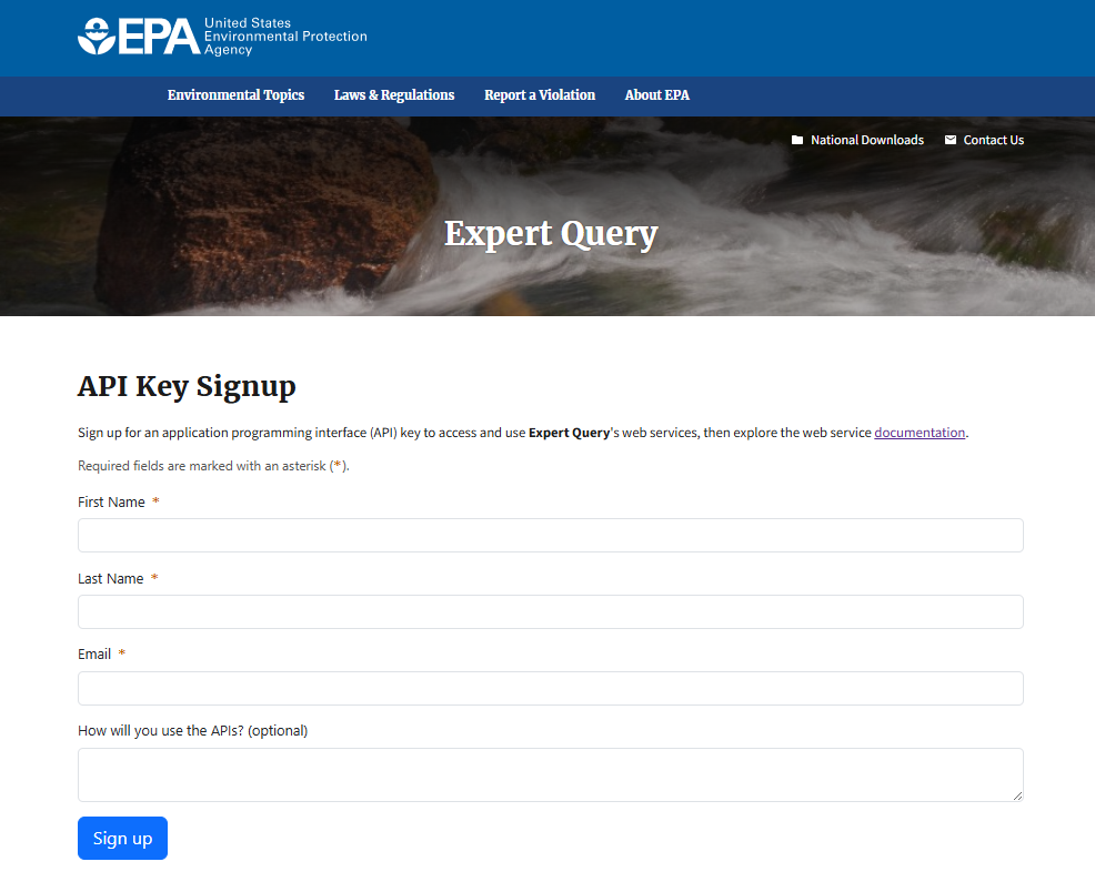
Some aspects of the Module 2 workflow depend on ATTAINS data imported via Expert Query web services. While public, Expert Query web services require an API key, a unique identifier used to authenticate access to the Expert Query API. The EPATADA package contains a default API key for Expert Query, so users who do not have their own API key can still use these functions.
However, Expert Query API keys are rate limited, meaning that if many users are all accessing Expert Query data using the same key at the same time, server failures from too many requests may occur. Best practice is for each EPATADA user is to obtain their own, individual API key by requesting one here: API Key Signup Form
If you have your own API key, uncomment the code below and assign your API key to the “api_key” variable. Otherwise, the default EPATADA package key will be used.
# api_key <- "paste your key here"

# is user does not provide key, set api_key as NULL
if (!exists("api_key")) {
  api_key <- NULL
}
Step A: Discover ML/AU Matches
The TADA_CreateAUMLCrosswalk function
efficiently creates a crosswalk between ATTAINS assessment units and WQP
monitoring locations. It uses three prioritized data sources:
User-Supplied Crosswalk: An optional crosswalk provided by the user (e.g., see example
user.supplied.cwin next code chunk).ATTAINS Crosswalk: Utilizes
TADA_GetATTAINSAUMLCrosswalkto incorporate crosswalk information stored by participating organizations in ATTAINS. There may not be an ATTAINS crosswalk available for all organizations as storing this information in ATTAINS is optional for states and some tribes are still in the process of developing their crosswalks.ATTAINS Catchments/Geospatial Join: Employs
TADA_CreateATTAINSAUMLCrosswalkto connect monitoring locations to assessment units using ATTAINS catchments through a geospatial join. This function converts WQP monitoring locations into a geospatial sf object and associates them with their intersecting NHDPlus high resolution catchments containing entity-defined assessment units in ATTAINS.
Process
The function prioritizes these sources in the order listed. It automatically attempts to assign unassigned monitoring locations using the next available data source. For example, if any monitoring locations remain unassigned after checking the user-supplied crosswalk, the function will check the ATTAINS crosswalk, then the geospatial join, as needed.
This entire process is automated within
TADA_CreateAUMLCrosswalk, so users do not need to run each step individually, though they have the option to do so if desired.To make this function run more efficiently, the default is to not return catchments from the ATTAINS geospatial service for matches found in the user-supplied crosswalk or ATTAINS crosswalk (#1 or #2 above). If the user does want to return ATTAINS geospatial service catchments for matches from the user-supplied or ATTAINS crosswalks, they can set fill_ATTAINS_catch = TRUE. This will return the catchments, but increases function run time significantly. ATTAINS catchments are always returned for
TADA_CreateATTAINSAUMLCrosswalkassessed WQP monitoring locations.
Create An Example User-Supplied Crosswalk
Get existing data from ATTAINS using
TADA_GetATTAINSAUMLCrosswalk and subset a few rows to
create an example user-supplied ATTAINS Assessment Unit and WQP
Monitoring Location crosswalk for demonstration purposes. If you have
your own crosswalk, this step can be skipped.
# review valid ATTAINS org IDs
ATTAINS_orgs <- rExpertQuery::EQ_DomainValues("org_id")

# get crosswalk from ATTAINS
attains.existing.MT <- TADA_GetATTAINSAUMLCrosswalk(
  org_id = "MTDEQ",
  api_key = api_key
)

# clean existing crosswalk from ATTAINS to make sure WQP monitoring location IDs pulled from ATTAINS are WQP compatible (adds org ID if missing)
clean.existing.attains.MT <- TADA_UpdateATTAINSAUMLCrosswalk(
  org_id = "MTDEQ",
  api_key = api_key
)

# create example user supplied crosswalk (select a few Monitoring Locations from the tada df to use in the example for demonstration purposes)
user.supplied.cw <- clean.existing.attains.MT |>
  dplyr::select(
    ATTAINS.AssessmentUnitIdentifier,
    ATTAINS.MonitoringLocationIdentifier,
    ATTAINS.WaterType
  ) |>
  dplyr::filter(ATTAINS.MonitoringLocationIdentifier %in% c(
    "MDEQ_WQ_WQX-C04CKFKR05", "MDEQ_WQ_WQX-C04KNDYC01", "MDEQ_WQ_WQX-C04KNDYC02",
    "MDEQ_WQ_WQX-C04KNDYC04", "MDEQ_WQ_WQX-C04KNDYC54"
  )) |>
  dplyr::rename(
    AssessmentUnitIdentifier = ATTAINS.AssessmentUnitIdentifier,
    MonitoringLocationIdentifier = ATTAINS.MonitoringLocationIdentifier,
    WaterType = ATTAINS.WaterType
  ) |>
  # Add an example new assessment unit for demonstration purposes
  dplyr::bind_rows(c(
    AssessmentUnitIdentifier = "NEW:EX_MDEQ_WQ_WQX",
    MonitoringLocationIdentifier = "NARS_WQX-NWC_MT-10184",
    WaterType = "LAKE, FRESHWATER"
  ))

rm(attains.existing.MT, clean.existing.attains.MT, ATTAINS_orgs)
Run TADA_CreateAUMLCrosswalk
# make AU assignments for unassigned MLs
MT.AUMLRef <- TADA_CreateAUMLCrosswalk(
  tada.MT.clean,
  au_ref = user.supplied.cw,
  org_id = "MTDEQ",
  fill_ATTAINS_catch = TRUE,
  return_nearest = TRUE,
  batch_upload = TRUE,
  api_key = api_key
)
# extract ATTAINS_crosswalk data frame from the list and show table
TADA_TableExport(MT.AUMLRef$ATTAINS_crosswalk)
Advanced: Deep Dive into
TADA_CreateATTAINSAUMLCrosswalk()
TADA_CreateAUMLCrosswalk() automatically runs
TADA_CreateATTAINSAUMLCrosswalk (see #3 under step A
above). This function pulls in ATTAINS data from the EPA’s ATTAINS
Assessment Geospatial Service and links it to TADA-pulled Water Quality
Portal observations. For the function to work properly, the input
dataframe must have - at a minimum - WQP observation coordinates in
“LongitudeMeasure” and “LatitudeMeasure” columns and a
“HorizontalCoordinateReferenceSystemDatumName” column.
By default, TADA_CreateATTAINSAUMLCrosswalk() returns a
dataframe with ATTAINS-linked Water Quality Portal entries. Users have
the added option of returning the intersecting ATTAINS geospatial
shapefile objects with their ATTAINS-linked Water Quality Portal
dataframe. If return_sf = TRUE, the function returns a list
containing the dataframe and shapefile objects named
ATTAINS_catchments, ATTAINS_lines,
ATTAINS_points, and ATTAINS_polygons. Note, if
any of these shapefile objects are empty, this indicates that there are
no ATTAINS objects of that type intersecting any WQP-linked ATTAINS
catchment.
Regardless of the user’s decision on returning the ATTAINS shapefile
objects, TADA_CreateATTAINSAUMLCrosswalk() always returns a
dataframe (or dataframes if fill_ATTAINS_catch = TRUE, see
section Filling in missing ATTAINS assessment units)
containing the original TADA WQP dataframe, plus new columns
representing the ATTAINS assessment unit(s) that fall within the same
NHDPlus HiRes catchment as them. This means that it is possible for a
single TADA WQP observation to have multiple ATTAINS assessment units
linked to it. If the user would like to link all of these features, set
return_nearest = FALSE. In these instances of multiple
assessment units in the same catchment, the returned dataframe will have
more than one row of data for each WQP observation. Such WQP
observations can be identified using the
ResultIdentifiercolumn (i.e., multiple rows with the same
ResultIdentifier value are the same observation).
To only return a single ATTAINS assessment unit, set
return_nearest = TRUE. This will return only the closest
assessment unit to the WQP observation in instances where a catchment
contains more than one assessment unit.
TADA_CreateATTAINSAUMLCrosswalk also runs
TADA_MakeSpatial() within it to convert any Water Quality
Portal (WQP)-style dataframe with latitude/longitude data into a
geospatial shapefile object. The user supplies a WQP dataframe and the
coordinate reference system that they want the spatial object to be in
[the default is CRS 4326 (WGS 84)]. For the function to work properly,
the input dataframe must have - at a minimum - WQP observation
coordinates in “LongitudeMeasure” and “LatitudeMeasure” and a
“HorizontalCoordinateReferenceSystemDatumName” column.
Let’s run TADA_MakeSpatial() to make the water quality
data spatial.
# Adds epsg and geometry column at end, uses default CRS WGS84 (4326)
TADA_spatial <- TADA_MakeSpatial(.data = tada.MT.clean, crs = 4326)
This new spatial object is identical to the original TADA dataframe,
but now includes a “geometry” column that allows for mapping and
additional geospatial capabilities. Enter ?TADA_MakeSpatial
into the console to review another example of this function in use and
additional information.
Now we can review the monitoring locations on a map:
leaflet::leaflet() |>
  leaflet::addProviderTiles("Esri.WorldTopoMap",
    group = "World topo",
    options = leaflet::providerTileOptions(
      updateWhenZooming = FALSE,
      updateWhenIdle = TRUE
    )
  ) |>
  leaflet::clearShapes() |>
  EPATADA:::addMapReset() |>
  leaflet::addLegend(
    position = "bottomright",
    colors = "black",
    labels = "Water Quality Observation(s)",
    opacity = 1
  ) |>
  leaflet::addCircleMarkers(
    data = TADA_spatial,
    color = "grey", fillColor = "black",
    fillOpacity = 0.8, stroke = TRUE, weight = 1.5, radius = 6,
    popup = paste0(
      "Site ID: ",
      TADA_spatial$MonitoringLocationIdentifier,
      "<br> Site Name: ",
      TADA_spatial$MonitoringLocationName
    )
  )
Using either our original tada.MT.clean or the
geospatial version TADA_spatial, we can pull in the ATTAINS
catchment features that intersect our observations:
TADA_with_ATTAINS <- TADA_CreateATTAINSAUMLCrosswalk(
  .data = tada.MT.clean,
  return_sf = FALSE,
  return_nearest = FALSE
)

# Can also be performed on the spatial data:
# TADA_with_ATTAINS <- TADA_CreateATTAINSAUMLCrosswalk(.data = TADA_spatial, return_sf = FALSE, return_nearest = TRUE)
This new TADA_with_ATTAINS object is a modification of
the original TADA Water Quality Portal dataframe that now has additional
columns associated with the ATTAINS assessment unit(s) that lie in the
same NHD HiRes catchment as them (these columns are prefixed with
“ATTAINS”). Moreover, because our TADA_with_ATTAINS object
contains more rows than the original TADA dataframe, we can deduce that
some Water Quality Portal observations fall within an NHD catchment that
contains more than one ATTAINS assessment unit.
TADA_with_ATTAINS_list <- TADA_CreateATTAINSAUMLCrosswalk(
  .data = tada.MT.clean,
  return_sf = TRUE,
  return_nearest = TRUE
)

# return only the closest ATTAINS AU for observations within a catchment with multiple AUs
# TADA_with_ATTAINS_list <- TADA_CreateATTAINSAUMLCrosswalk(.data = TADA_spatial, return_sf = TRUE, return_nearest = TRUE)
If we set return_sf = TRUE as done to create the
TADA_with_ATTAINS_list object above, we also now have all
the raw intersecting ATTAINS features associated with these ATTAINS
catchment observations stored in a list along with the TADA
dataframe.
Arguments for
TADA_CreateATTAINSAUMLCrosswalk()
.data: Your input TADA-style Water Quality Portal data.return_nearest: If TRUE, returns only the nearest ATTAINS feature to each WQP observation.return_sf: If TRUE, returns spatial data in addition to tabular data.
Step B: Review MLs/AUs on a Map
The TADA_ViewATTAINS() function creates
a map that visually represents the monitoring locations and assessment
units. When the param ref_icons is equal to TRUE, the results from the
three different crosswalk sources are shown using distinct circle marker
icons:
User-Supplied Crosswalk: Monitoring locations derived from a user-supplied reference are indicated by a user icon.
ATTAINS Crosswalk: Locations that match with the crosswalk downloaded from ATTAINS are marked with a circle that contains a check mark.
ATTAINS Catchments/Geospatial Join: Matches found by joining monitoring locations with ATTAINS catchments in
TADA_CreateATTAINSAUMLCrosswalk()whenreturn_sf = TRUEare shown as solid fill circle markers.
Additionally, when a user clicks on any circle marker, a pop-up window appears displaying the assessment unit crosswalk source for that particular monitoring location.
Alternately, users can set ref_icons equal to FALSE to display all monitoring locations as plain circle markers regardless of the crosswalk source.
Let’s view the data associated with MT.AUMLRef!
TADA_ViewATTAINS(MT.AUMLRef, ref_icons = TRUE)Enter ?TADA_ViewATTAINS into the console to review
another example of this function in use and additional information.
Step C: Upload ML/AU crosswalk to ATTAINS
The TADA_UpdateATTAINSAUMLCrosswalk
function generates an output that can be batch uploaded to ATTAINS,
enabling the creation or updating of Monitoring Location Identifiers
within ATTAINS Assessment Unit profiles.
Workflow Example:
Access the Element:
Begin by accessing theATTAINS_batchuploadelement from the list generated by theTADA_CreateAUMLCrosswalkfunction (e.g. MT.AUMLRef).Review and Modify:
Review theATTAINS_batchuploadelement and make any necessary modifications.Execute the Function:
ExecuteTADA_UpdateATTAINSAUMLCrosswalk. This process adds new links to WQP site pages, preparing the data for upload to ATTAINS.-
Choose Update Option:
When runningTADA_UpdateATTAINSAUMLCrosswalk(), with theattains_replacefunction input users have the option to:Overwrite: Replace all existing records.
Append: Add new Monitoring Location Identifiers to the current records.
For more detailed instructions, enter
?TADA_UpdateATTAINSAUMLCrosswalk into the console.
batch.upload.MT <- MT.AUMLRef$ATTAINS_batchupload |>
  TADA_UpdateATTAINSAUMLCrosswalk( # selected attains_replace = TRUE because all matches currently in ATTAINS are included in this new crosswalk
    attains_replace = TRUE,
    batch_upload = TRUE,
    wqp_data_links = "add",
    # ml ids have already  been corrected if needed
    update_mlid = FALSE,
    org_id = "MTDEQ",
    api_key = api_key
  )
Step D: Assign Uses to AUs
After mapping the WQP monitoring locations (MLs) to ATTAINS
assessment units (AUs), we will use the TADA_AssignUsesToAU
function to assign specific uses to these assessment units.
Additionally, we will demonstrate how to automatically assign uses to
the new assessment unit, NEW:EX_MDEQ_WQ_WQX with the water
type “LAKE, FRESHWATER,” that was created in step A, which is not yet
present in ATTAINS.
# extract ATTAINS_crosswalk data frame from the list
Final.MT.AUMLRef <- MT.AUMLRef$ATTAINS_crosswalk

# this is the same final output we got above from TADA_CreateAUMLCrosswalk
TADA_TableExport(Final.MT.AUMLRef)
Now, we will assign uses to each unique assessment unit (AU) in our
finalized monitoring location to assessment unit crosswalk (e.g.,
Final.MT.AUMLRef). The process of assigning uses to AUs
follows these prioritized steps:
User-Supplied Crosswalk (Optional): Utilize a crosswalk provided by the user that maps specific uses to assessment units.
Existing Uses from ATTAINS: Import existing uses for assessment units as defined by ATTAINS organizations.
MT.UseAURef <- TADA_AssignUsesToAU(
  MT.AUMLRef$TADA_with_ATTAINS,
  AUMLRef = Final.MT.AUMLRef,
  org_id = "MTDEQ",
  api_key = api_key
)
TADA_TableExport(MT.UseAURef)Advanced: Assigning Uses to New AUs
For any new assessment unit (AU), users must determine how to assign
the appropriate uses. The
TADA_AssignUsesToWaterType function is
designed to assist with this process. It imports combinations of water
types and use names associated with the specified organization from
ATTAINS. By doing so, it automatically assigns uses to new assessment
units based on their water type, thereby streamlining the integration of
new AUs into existing frameworks.
For more information on how to customize this function to suit your
needs, enter ?TADA_AssignUsesToWaterType
into the R console.
MT.UseAURef_with_WaterUseRef <-
  TADA_AssignUsesToAU(
    MT.AUMLRef$TADA_with_ATTAINS,
    waterUseRef = TADA_AssignUsesToWaterType(org_id = "MTDEQ"),
    AUMLRef = Final.MT.AUMLRef,
    org_id = "MTDEQ",
    api_key = api_key
  )
TADA_TableExport(MT.UseAURef_with_WaterUseRef)Users also have the option to manually assign use names to new AUs if they prefer not to use the TADA_AssignUsesToWaterType function. This approach allows for greater flexibility and customization when integrating new AUs into existing frameworks.
MT.UseAURef_manual <- MT.UseAURef |>
  dplyr::left_join(
    data.frame(
      ATTAINS.UseName = c("Aquatic Life", "Drinking Water"),
      ATTAINS.AssessmentUnitIdentifier = c("NEW:EX_MDEQ_WQ_WQX", "NEW:EX_MDEQ_WQ_WQX")
    ),
    by = ("ATTAINS.AssessmentUnitIdentifier")
  ) |>
  dplyr::mutate(ATTAINS.UseName = dplyr::coalesce(ATTAINS.UseName.x, ATTAINS.UseName.y)) |>
  dplyr::select(-ATTAINS.UseName.x, -ATTAINS.UseName.y)

TADA_TableExport(MT.UseAURef_manual)
Summary
In conclusion, this example TADA Module 2 workflow significantly enhances the ability to maintain up-to-date information on WQP Monitoring Locations and the uses being assessed at various ATTAINS Assessment Units. By systematically guiding users through the creation of crosswalks, map reviews, data submission, and use assignments, this workflow supports efficient data management and improves reproducibility.