TADA Module 1: Training for Intermediate/Advanced R Users
TADA Team
2026-07-24
Source:vignettes/TADAModule1_AdvancedTraining.Rmd
TADAModule1_AdvancedTraining.RmdWelcome!
Thank you for your interest in Tools for Automated Data Analysis (TADA). TADA is an open-source tool set built in the R programming language and available for anyone to download and edit to their specific needs. This TADA Module 1: Training for Intermediate/Advanced R Users RMarkdown document (learn more about RMarkdown) walks through how to download the TADA R package from GitHub, access and parameterize several important functions with a sample dataframe, and create basic visualizations.
The workflow is similar to a funnel: at each decision point, data that fail QC checks are removed from the core dataframe and placed in a separate dataframe, while data that pass are carried into the next step. At the end of the QC checks, the user should be confident that their data are properly documented and applicable to the analysis at hand.
Note: TADA is still under development. New functionality is added weekly, and sometimes we need to make bug fixes in response to tester and user feedback. We appreciate your feedback, patience, and interest in these helpful tools.
Customize or contribute
TADA is housed in a repository on GitHub. Users desiring to review the base code and customize the package for their own purposes may:
Clone the repository using Git
Open the repository using GitHub Desktop, or
Download a zip file of the repository to their desktop.
Interested in contributing to the TADA package? The TADA team highly encourages input and development from users. Check out the Contributing page on the TADA GitHub site for guidance on collaboration conventions.
Install and load packages
First, install and load the remotes package specifying the repo. This is needed before installing EPATADA because it is only available on GitHub (not CRAN).
install.packages("remotes",
repos = "http://cran.us.r-project.org"
)
library(remotes)Next, install and load EPATADA using the remotes package. USGS’s dataRetrieval and other TADA R Package dependencies will also be downloaded automatically from CRAN with the TADA install. If desired, the development version of dataRetrieval can be downloaded directly from GitHub (un-comment).
remotes::install_github("USEPA/EPATADA",
ref = "develop",
dependencies = TRUE
)
# remotes::install_github("USGS-R/dataRetrieval", dependencies=TRUE)Finally, use the library() function to load the TADA R Package into your R session.
Help pages
All TADA R package functions have their own individual help pages,
listed on the Function
reference page on the GitHub site. Users can also access the help
page for a given function in R or RStudio using the following format
(example below): ?[name of TADA function]
?TADA_DataRetrievalUpload data
Now let’s start using the TADA R package functions. The first step is to bring a dataframe into the R environment. TADA is designed to work with Water Quality Portal (WQP) data. This means that all of its functions will look for WQP column names and create new TADA-specific columns based on these elements. Users may upload their own custom dataframe into R for use with TADA by ensuring their column names and data formats (e.g. numeric, character) align with WQP profiles.
If you are interested in reviewing the column headers and formats required to run TADA, use the function below.
template <- TADA_GetTemplate()
template## [1] ResultIdentifier
## [2] ActivityTypeCode
## [3] ActivityMediaName
## [4] ActivityMediaSubdivisionName
## [5] CountryCode
## [6] StateCode
## [7] CountyCode
## [8] MonitoringLocationName
## [9] MonitoringLocationTypeName
## [10] MonitoringLocationDescriptionText
## [11] LatitudeMeasure
## [12] LongitudeMeasure
## [13] HorizontalCoordinateReferenceSystemDatumName
## [14] HUCEightDigitCode
## [15] MonitoringLocationIdentifier
## [16] ResultSampleFractionText
## [17] CharacteristicName
## [18] SubjectTaxonomicName
## [19] MethodSpeciationName
## [20] ActivityStartDate
## [21] ActivityStartTime.Time
## [22] ActivityStartTime.TimeZoneCode
## [23] ActivityStartDateTime
## [24] ResultMeasureValue
## [25] ResultMeasure.MeasureUnitCode
## [26] ResultValueTypeName
## [27] ResultDetectionConditionText
## [28] DetectionQuantitationLimitTypeName
## [29] DetectionQuantitationLimitMeasure.MeasureValue
## [30] DetectionQuantitationLimitMeasure.MeasureUnitCode
## [31] ResultDepthHeightMeasure.MeasureValue
## [32] ResultDepthHeightMeasure.MeasureUnitCode
## [33] ResultDepthAltitudeReferencePointText
## [34] ActivityRelativeDepthName
## [35] ActivityDepthHeightMeasure.MeasureValue
## [36] ActivityDepthHeightMeasure.MeasureUnitCode
## [37] ActivityTopDepthHeightMeasure.MeasureValue
## [38] ActivityTopDepthHeightMeasure.MeasureUnitCode
## [39] ActivityBottomDepthHeightMeasure.MeasureValue
## [40] ActivityBottomDepthHeightMeasure.MeasureUnitCode
## [41] ResultTimeBasisText
## [42] StatisticalBaseCode
## [43] ResultFileUrl
## [44] ResultAnalyticalMethod.MethodName
## [45] ResultAnalyticalMethod.MethodDescriptionText
## [46] ResultAnalyticalMethod.MethodIdentifier
## [47] ResultAnalyticalMethod.MethodIdentifierContext
## [48] ResultAnalyticalMethod.MethodUrl
## [49] SampleCollectionMethod.MethodIdentifier
## [50] SampleCollectionMethod.MethodIdentifierContext
## [51] SampleCollectionMethod.MethodName
## [52] SampleCollectionMethod.MethodDescriptionText
## [53] SampleCollectionEquipmentName
## [54] MeasureQualifierCode
## [55] ResultStatusIdentifier
## [56] ResultCommentText
## [57] ActivityCommentText
## [58] HydrologicCondition
## [59] HydrologicEvent
## [60] DataQuality.PrecisionValue
## [61] DataQuality.BiasValue
## [62] DataQuality.ConfidenceIntervalValue
## [63] DataQuality.UpperConfidenceLimitValue
## [64] DataQuality.LowerConfidenceLimitValue
## [65] SamplingDesignTypeCode
## [66] LaboratoryName
## [67] ResultLaboratoryCommentText
## [68] ActivityIdentifier
## [69] OrganizationIdentifier
## [70] OrganizationFormalName
## [71] ProjectName
## [72] ProjectDescriptionText
## [73] ProjectIdentifier
## [74] ProjectFileUrl
## [75] QAPPApprovedIndicator
## [76] QAPPApprovalAgencyName
## [77] AquiferName
## [78] AquiferTypeName
## [79] LocalAqfrName
## [80] ConstructionDateText
## [81] WellDepthMeasure.MeasureValue
## [82] WellDepthMeasure.MeasureUnitCode
## [83] WellHoleDepthMeasure.MeasureValue
## [84] WellHoleDepthMeasure.MeasureUnitCode
## [85] ProviderName
## [86] LastUpdated
## <0 rows> (or 0-length row.names)TADA_DataRetrieval is built upon USGS’s
dataRetrieval::readWQPdata and
dataRetrieval::whatWQPsites functions within the
dataRetrieval package, which uses web service calls to bring WQP data
into the R environment. Additionally, TADA_DataRetrieval
performs some basic quality control checks via
TADA_AutoClean on the data using new TADA-specific columns
to preserve the original dataframe:
Converts key character columns to ALL CAPS for easier harmonization and validation.
Identifies different classes of result values (numeric, text, percentage, comma-separated numeric, greater than/less than, numbers preceded by a tilde, etc.) and converts values to numeric where feasible.
Unifies result and depth units to common units to improve ease of data harmonization. See
?TADA_ConvertResultUnitsand?TADA_ConvertDepthUnitsfor more information on these processes. These functions can also be run separately if the user wishes to convert result or depth values to different units.
Let’s give it a try. Setting applyautoclean to TRUE in
TADA:TADA_DataRetrieval means that the basic quality
control steps described above are run. See ?TADA_AutoClean
for more details. TADA_DataRetrieval follows similar
parameterization to the dataRetrieval package function
dataRetrieval::readWQPdata, but check out the help
page or enter ?TADA_DataRetrieval into the console for
more information about input parameters and to see several examples.
# download example data
# dataset_0 <- TADA_DataRetrieval(
# organization = c(
# "REDLAKE_WQX", # Red Lake Band of Chippewa Indians
# "FONDULAC_WQX", # Minnesota Chippewa Tribe (Fond du Lac Band)
# "PUEBLOOFTESUQUE", # Pueblo of Tesuque
# "PENOBSCOTINDIANNATIONDNR", # Penobscot Indian Nation
# "UTEMTN", # Ute Mountain Ute Tribe
# "BLCKFEET" # Blackfeet Nation
# ),
# # last 20 years
# startDate = "2005-01-01",
# endDate = "2025-12-31",
# ask = TRUE
# )
# For brevity, we'll skip pinging the WQP and instead load the example dataframe:
dataset_0 <- Data_TribalNationsLet’s take a look at all of the TADA-created columns:
## [1] "TADA.ActivityMediaName"
## [2] "TADA.MonitoringLocationName"
## [3] "TADA.MonitoringLocationTypeName"
## [4] "TADA.LatitudeMeasure"
## [5] "TADA.LongitudeMeasure"
## [6] "TADA.MonitoringLocationIdentifier"
## [7] "TADA.ResultSampleFractionText"
## [8] "TADA.CharacteristicName"
## [9] "TADA.MethodSpeciationName"
## [10] "TADA.ComparableDataIdentifier"
## [11] "TADA.ResultMeasureValue"
## [12] "TADA.ResultMeasure.MeasureUnitCode"
## [13] "TADA.WQXResultUnitConversion"
## [14] "TADA.ResultMeasureValueDataTypes.Flag"
## [15] "TADA.DetectionQuantitationLimitMeasure.MeasureValue"
## [16] "TADA.DetectionQuantitationLimitMeasure.MeasureUnitCode"
## [17] "TADA.DetectionQuantitationLimitMeasure.MeasureValueDataTypes.Flag"
## [18] "TADA.ResultDepthHeightMeasure.MeasureValue"
## [19] "TADA.ResultDepthHeightMeasure.MeasureValueDataTypes.Flag"
## [20] "TADA.ResultDepthHeightMeasure.MeasureUnitCode"
## [21] "TADA.ActivityDepthHeightMeasure.MeasureValue"
## [22] "TADA.ActivityDepthHeightMeasure.MeasureValueDataTypes.Flag"
## [23] "TADA.ActivityDepthHeightMeasure.MeasureUnitCode"
## [24] "TADA.ActivityTopDepthHeightMeasure.MeasureValue"
## [25] "TADA.ActivityTopDepthHeightMeasure.MeasureValueDataTypes.Flag"
## [26] "TADA.ActivityTopDepthHeightMeasure.MeasureUnitCode"
## [27] "TADA.ActivityBottomDepthHeightMeasure.MeasureValue"
## [28] "TADA.ActivityBottomDepthHeightMeasure.MeasureValueDataTypes.Flag"
## [29] "TADA.ActivityBottomDepthHeightMeasure.MeasureUnitCode"Currently, the TADA_DataRetrieval function combines
three WQP data profiles: Sample Results (Physical/Chemical), Site data,
and Project data. This ensures that all important quality control
columns are included in the dataframe.
Note: USGS and EPA are working together to create
WQP 3.0 data profiles. Once released (coming in 2025), one data profile
will contain the columns critical to TADA, removing the need to combine
profiles in this first step. This will simplify the steps needed to
upload a custom or WQP GUI-downloaded dataframe into the R package.
However, column names are changing in the new WQP 3.0 data profiles.
This will impact the TADA_DataRetrieval function. The WQP
and TADA teams are available to assist with cross walking the old to new
column names when the time comes.
Initial data review
Now that we’ve pulled the data into the R session, let’s take a look
at it. Note that any column names with the “TADA.” prefix were generated
from the TADA_DataRetrieval function.
First, always good to take a look at the dataframe dimensions.
Question 1: What are the dimensions of your dataframe?
dim(dataset_0) # returns x and of x (as the numbers of rows and columns respectively)## [1] 143119 152Before we start filtering and flagging our data, let’s create a
function (dimCheck) that performs dimension checks between
the results that pass each filter or QC flag check (and are retained)
and those that do not (and are removed). These dimension checks ensure
that the total number of rows in the original input dataframe
(all_result_num) equal the the total number of rows added
up between the passing (pass_data) and removed
(fail_data) dataframes.
# defining a dimension check function that compares removed and retained data dimensions against the initial data input
dimCheck <- function(all_result_num, pass_data, fail_data, checkName) {
# check result numbers after split
final_result_num <- dim(pass_data)[1] + dim(fail_data)[1]
# always good to do a dimension check
if (!all_result_num == final_result_num) {
print(paste0("Help! Results do not add up between dataframe and removed after ", checkName, " check."))
} else {
print(paste0("Good to go. Zero results created or destroyed in ", checkName, " check."))
}
}
# let's first get the total number of rows in the dataframe.
all_result_num <- dim(dataset_0)[1]Next, we can use the TADA_FieldCounts() function to see
how many unique values are contained within each column of the
dataframe. The function can either return all column counts, most, or
just the key columns. We’ll try the input with
display = "key" and display = "all". Enter
?TADA_FieldCounts() into the console for more information
on this function.
Question 2: Which column should have a unique value in every row and why?
key_counts <- TADA_FieldCounts(dataset_0, display = "key")
key_counts## Fields Count
## 1 TADA.ComparableDataIdentifier 309
## 2 SubjectTaxonomicName 307
## 3 TADA.CharacteristicName 223
## 4 TADA.MonitoringLocationTypeName 8
## 5 OrganizationFormalName 5
## 6 TADA.ActivityMediaName 3
## 7 ActivityMediaSubdivisionName 3
## 8 ActivityRelativeDepthName 3
## 9 ResultValueTypeName 3
## 10 ResultStatusIdentifier 2
## 11 HydrologicCondition 1
## 12 HydrologicEvent 1
## 13 SampleTissueAnatomyName 1
all_counts <- TADA_FieldCounts(dataset_0, display = "all")
all_counts## Fields Count
## 1 ResultIdentifier 143119
## 2 TADA.ResultMeasureValue 44218
## 3 ResultMeasureValue 42595
## 4 ActivityIdentifier 17547
## 5 ResultDetectionQuantitationLimitUrl 12228
## 6 ActivityStartDateTime 10734
## 7 LastUpdated 3502
## 8 ResultDepthHeightMeasure.MeasureValue 3006
## 9 TADA.ResultDepthHeightMeasure.MeasureValue 3006
## 10 ActivityCommentText 1922
## 11 ActivityStartTime.Time 1350
## 12 ActivityDepthHeightMeasure.MeasureValue 1155
## 13 TADA.ActivityDepthHeightMeasure.MeasureValue 1155
## 14 ActivityStartDate 671
## 15 AnalysisStartDate 568
## 16 ActivityLocation.LongitudeMeasure 465
## 17 ActivityLocation.LatitudeMeasure 460
## 18 TADA.DetectionQuantitationLimitMeasure.MeasureValue 390
## 19 DetectionQuantitationLimitMeasure.MeasureValue 380
## 20 ResultCommentText 330
## 21 TADA.ComparableDataIdentifier 309
## 22 SubjectTaxonomicName 307
## 23 ActivityEndDate 251
## 24 ActivityEndDateTime 251
## 25 MonitoringLocationIdentifier 231
## 26 TADA.MonitoringLocationIdentifier 231
## 27 MonitoringLocationName 230
## 28 TADA.MonitoringLocationName 230
## 29 LongitudeMeasure 224
## 30 TADA.LongitudeMeasure 224
## 31 CharacteristicName 224
## 32 TADA.CharacteristicName 223
## 33 LatitudeMeasure 221
## 34 TADA.LatitudeMeasure 221
## 35 MonitoringLocationDescriptionText 80
## 36 ResultAnalyticalMethod.MethodName 78
## 37 ResultAnalyticalMethod.MethodIdentifier 76
## 38 VerticalMeasure.MeasureValue 68
## 39 ResultAnalyticalMethod.MethodDescriptionText 45
## 40 ResultMeasure.MeasureUnitCode 42
## 41 ActivityBottomDepthHeightMeasure.MeasureValue 35
## 42 TADA.ActivityBottomDepthHeightMeasure.MeasureValue 35
## 43 ProjectName 25
## 44 ProjectIdentifier 25
## 45 TADA.ResultMeasure.MeasureUnitCode 22
## 46 HUCEightDigitCode 17
## 47 ResultAnalyticalMethod.MethodIdentifierContext 15
## 48 CountyCode 14
## 49 SampleCollectionMethod.MethodIdentifier 14
## 50 SampleCollectionMethod.MethodName 14
## 51 SampleCollectionMethod.MethodDescriptionText 14
## 52 LaboratoryName 14
## 53 ProjectDescriptionText 13
## 54 DetectionQuantitationLimitMeasure.MeasureUnitCode 11
## 55 TADA.DetectionQuantitationLimitMeasure.MeasureUnitCode 10
## 56 ActivityTypeCode 9
## 57 TADA.ResultMeasureValueDataTypes.Flag 9
## 58 SampleCollectionEquipmentName 9
## 59 MeasureQualifierCode 9
## 60 MonitoringLocationTypeName 8
## 61 TADA.MonitoringLocationTypeName 8
## 62 ResultSampleFractionText 8
## 63 MethodSpeciationName 8
## 64 TADA.ResultSampleFractionText 7
## 65 TADA.MethodSpeciationName 7
## 66 ResultDetectionConditionText 7
## 67 DetectionQuantitationLimitTypeName 7
## 68 StateCode 6
## 69 SampleCollectionMethod.MethodIdentifierContext 6
## 70 DataQuality.UpperConfidenceLimitValue 6
## 71 DataQuality.LowerConfidenceLimitValue 6
## 72 ActivityStartTime.TimeZoneCode 5
## 73 StatisticalBaseCode 5
## 74 OrganizationIdentifier 5
## 75 OrganizationFormalName 5
## 76 HorizontalCollectionMethodName 5
## 77 ActivityStartTime.TimeZoneCode_offset 4
## 78 QAPPApprovedIndicator 4
## 79 QAPPApprovalAgencyName 4
## 80 VerticalCollectionMethodName 4
## 81 ActivityMediaName 3
## 82 TADA.ActivityMediaName 3
## 83 ActivityMediaSubdivisionName 3
## 84 HorizontalCoordinateReferenceSystemDatumName 3
## 85 TADA.WQXResultUnitConversion 3
## 86 ResultValueTypeName 3
## 87 ResultDepthHeightMeasure.MeasureUnitCode 3
## 88 ActivityRelativeDepthName 3
## 89 TADA.ActivityDepthHeightMeasure.MeasureValueDataTypes.Flag 3
## 90 ActivityDepthHeightMeasure.MeasureUnitCode 3
## 91 TADA.ActivityBottomDepthHeightMeasure.MeasureValueDataTypes.Flag 3
## 92 ActivityEndTime.TimeZoneCode 3
## 93 ActivityEndTime.TimeZoneCode_offset 3
## 94 VerticalMeasure.MeasureUnitCode 3
## 95 CountryCode 2
## 96 TADA.DetectionQuantitationLimitMeasure.MeasureValueDataTypes.Flag 2
## 97 TADA.ResultDepthHeightMeasure.MeasureValueDataTypes.Flag 2
## 98 ActivityTopDepthHeightMeasure.MeasureValue 2
## 99 TADA.ActivityTopDepthHeightMeasure.MeasureValue 2
## 100 TADA.ActivityTopDepthHeightMeasure.MeasureValueDataTypes.Flag 2
## 101 ActivityTopDepthHeightMeasure.MeasureUnitCode 2
## 102 ActivityBottomDepthHeightMeasure.MeasureUnitCode 2
## 103 ResultTimeBasisText 2
## 104 ResultStatusIdentifier 2
## 105 SamplingDesignTypeCode 2
## 106 ProjectFileUrl 2
## 107 ActivityEndTime.Time 2
## 108 VerticalCoordinateReferenceSystemDatumName 2
## 109 ProjectMonitoringLocationWeightingUrl 2
## 110 TADA.ResultDepthHeightMeasure.MeasureUnitCode 1
## 111 ResultDepthAltitudeReferencePointText 1
## 112 TADA.ActivityDepthHeightMeasure.MeasureUnitCode 1
## 113 TADA.ActivityTopDepthHeightMeasure.MeasureUnitCode 1
## 114 TADA.ActivityBottomDepthHeightMeasure.MeasureUnitCode 1
## 115 ResultFileUrl 1
## 116 ResultAnalyticalMethod.MethodUrl 1
## 117 HydrologicCondition 1
## 118 HydrologicEvent 1
## 119 ResultLaboratoryCommentText 1
## 120 AquiferName 1
## 121 AquiferTypeName 1
## 122 LocalAqfrName 1
## 123 WellDepthMeasure.MeasureUnitCode 1
## 124 WellHoleDepthMeasure.MeasureUnitCode 1
## 125 ProviderName 1
## 126 ActivityDepthAltitudeReferencePointText 1
## 127 ActivityConductingOrganizationText 1
## 128 SampleAquifer 1
## 129 ResultWeightBasisText 1
## 130 ResultTemperatureBasisText 1
## 131 ResultParticleSizeBasisText 1
## 132 USGSPCode 1
## 133 BinaryObjectFileName 1
## 134 BinaryObjectFileTypeCode 1
## 135 LabSamplePreparationUrl 1
## 136 SourceMapScaleNumeric 1
## 137 HorizontalAccuracyMeasure.MeasureUnitCode 1
## 138 VerticalAccuracyMeasure.MeasureUnitCode 1
## 139 FormationTypeText 1
## 140 DrainageAreaMeasure.MeasureUnitCode 1
## 141 ContributingDrainageAreaMeasure.MeasureUnitCode 1
## 142 SampleTissueAnatomyName 1Question 3: How many unique ‘TADA.ActivityMediaName’ values exist in your dataframe? Are there any media types that are not water?
TADA is currently designed to accommodate water data from the WQP. Let’s ensure that we remove all non-water data first.
# remove data with media type that is not water
removed <- dataset_0 |>
dplyr::filter(!TADA.ActivityMediaName %in% c("WATER")) |>
dplyr::mutate(TADA.RemovalReason = "Activity media is not water.")
# what other media types exist in dataframe?
unique(removed$TADA.ActivityMediaName)## [1] "BIOLOGICAL" "HABITAT"
# clean dataframe containing only water
dataset <- dataset_0 |> dplyr::filter(TADA.ActivityMediaName %in% c("WATER"))
dimCheck(all_result_num, dataset, removed, checkName = "Activity Media")## [1] "Good to go. Zero results created or destroyed in Activity Media check."Two additional helper functions one can use at any step in the
process are TADA_FieldValuesTable() and
TADA_FieldValuesPie(). These functions create a summary
table and pie chart (respectively) of all the unique values in a given
column. Let’s give it a try on OrganizationFormalName, which is a WQP
column naming the organization that supplied the result.
TADA_FieldValuesPie(dataset, field = "OrganizationFormalName")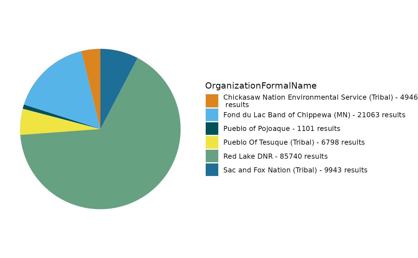
org_counts <- TADA_FieldValuesTable(dataset, field = "OrganizationFormalName")
org_counts## Value Count
## 1 Red Lake DNR 84965
## 2 Fond du Lac Band of Chippewa (MN) 27928
## 3 Blackfeet Nation (Montana) 20126
## 4 Ute Mountain Utes Tribe (Colorado) (Tribal) 4257
## 5 Pueblo Of Tesuque (Tribal) 793Question 4: When might a user choose to view a column’s unique values as a table rather than in a pie chart?
We can take a quick look at some of the TADA-created columns that
review result value types. Because TADA is intended to work with numeric
data, at this point, it would be good to remove those result values that
are NA without any detection limit info, or contain text or special
characters that cannot be converted to numeric. Note that TADA will fill
in missing values with detection limit values and units with the
TADA_IDCensoredData if the ResultDetectionConditionText and
DetectionQuantitationLimitType fields are populated. See
?TADA_ConvertSpecialChars for more details on result value
types and handling and ?TADA_IDCensoredData for details on
censored data preparation.
First, we can run TADA_IDCensoredData to fill in as many
NA/missing values as possible. We can use
TADA_FieldValuesPie to view the censored data flags
identified in the dataframe and their relative frequency.
TADA_IDCensoredData sorts result values into detection
limit categories (e.g. non-detect, over-detect) based on populated
values in the ResultDetectionConditionText and
DetectionQuantitationLimitTypeName columns.
You can find the reference tables used to make these decisions in
TADA_GetDetCondRef() and TADA_GetDetLimitRef()
functions. In some cases, results are missing detection limit/condition
info, or there is a conflict in the detection limit and condition. The
user may want to remove problematic detection limit data before
proceeding. We can also filter for the “problem” data by
TADA.CensoredData.Flag and review the unique reasons for data
removal.
dataset <- TADA_IDCensoredData(dataset)
TADA_FieldValuesPie(dataset, field = "TADA.CensoredData.Flag")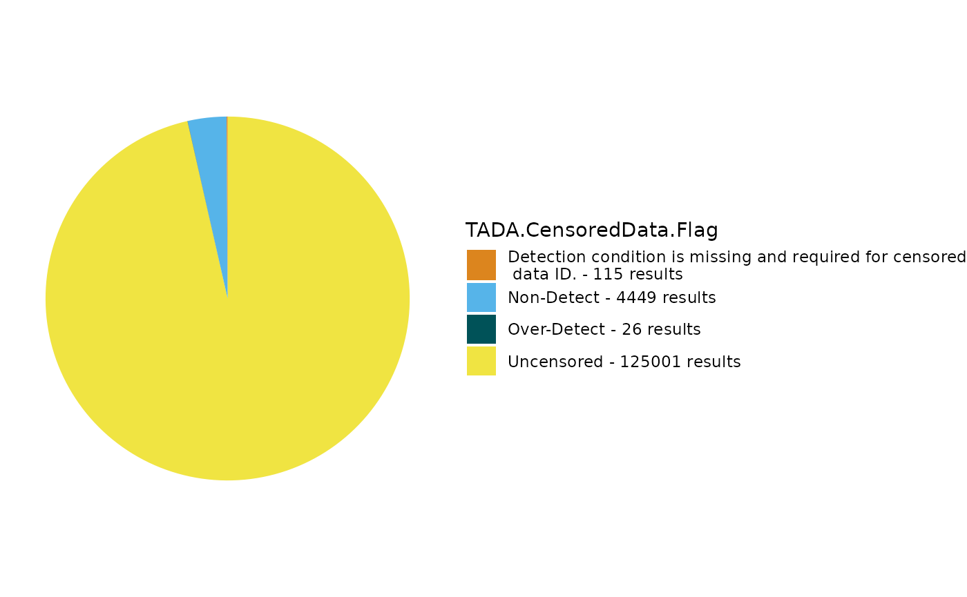
problem_censored <- dataset |>
dplyr::filter(!TADA.CensoredData.Flag %in% c("Non-Detect", "Over-Detect", "Other", "Uncensored")) |>
dplyr::mutate(TADA.RemovalReason = "Detection limit information contains errors or missing information.")
# Let's take a look at the problematic data that we filtered out (if any)
check <- unique(problem_censored[, c("TADA.CharacteristicName", "ResultDetectionConditionText", "DetectionQuantitationLimitTypeName", "TADA.CensoredData.Flag")])
TADA_TableExport(check)
dataset <- dataset |> dplyr::filter(TADA.CensoredData.Flag %in% c("Non-Detect", "Over-Detect", "Other", "Uncensored"))
# Let's take a look at the removed data
removed <- plyr::rbind.fill(removed, problem_censored)
# dimension check
dimCheck(all_result_num, dataset, removed, checkName = "Censored Data")Next, we can take a look at the data types present and filter out any non-allowable types.
# take a look at datatypes
flag.datatypes <- TADA_FieldValuesTable(dataset, field = "TADA.ResultMeasureValueDataTypes.Flag")
# Numeric or numeric-coerced data types
rv_datatypes <- unique(subset(dataset, !is.na(dataset$TADA.ResultMeasureValue))$TADA.ResultMeasureValueDataTypes.Flag)
# Non-numeric data types coerced to NA
na_rv_datatypes <- unique(subset(dataset, is.na(dataset$TADA.ResultMeasureValue))$TADA.ResultMeasureValueDataTypes.Flag)
# these are all of the NOT allowable data types in the dataset.
incompatible_datatype <- dataset |>
dplyr::filter(!dataset$TADA.ResultMeasureValueDataTypes.Flag %in% c("Numeric", "Less Than", "Greater Than", "Approximate Value", "Percentage", "Comma-Separated Numeric", "Numeric Range - Averaged", "Result Value/Unit Copied from Detection Limit")) |>
dplyr::mutate(TADA.RemovalReason = "Result value type cannot be converted to numeric or no detection limit values provided.")
# take a look at the difficult data types - do they make sense?
check <- unique(incompatible_datatype[, c("TADA.CharacteristicName", "ResultMeasureValue", "TADA.ResultMeasureValue", "ResultMeasure.MeasureUnitCode", "TADA.ResultMeasure.MeasureUnitCode", "TADA.ResultMeasureValueDataTypes.Flag", "DetectionQuantitationLimitMeasure.MeasureValue", "TADA.DetectionQuantitationLimitMeasure.MeasureValue", "DetectionQuantitationLimitMeasure.MeasureUnitCode", "TADA.DetectionQuantitationLimitMeasure.MeasureUnitCode")])
TADA_TableExport(check)Then we can take a closer look at the removed results and run another dimension check on the data set.
# filter data set to include allowable data types
dataset <- dataset |> dplyr::filter(dataset$TADA.ResultMeasureValueDataTypes.Flag %in% c("Numeric", "Less Than", "Greater Than", "Approximate Value", "Percentage", "Comma-Separated Numeric", "Numeric Range - Averaged", "Result Value/Unit Copied from Detection Limit"))
# create dataframe to includ all removed results
removed <- plyr::rbind.fill(removed, incompatible_datatype)
# dimension check
dimCheck(all_result_num, dataset, removed, checkName = "Result Format")## [1] "Good to go. Zero results created or destroyed in Result Format check."Data flagging
We’ve taken a quick look at the raw dataframe and split off some data
that are not compatible with TADA, now let’s run through some quality
control checks. The most important ones to run to ensure your dataframe
is ready for subsequent steps are TADA_FlagFraction(),
TADA_FlagSpeciation(), TADA_FlagResultUnit(),
and TADA_FindQCActivities(). With the exception of
TADA_FindQCActivities(), these flagging functions leverage
WQX’s QAQC
Validation Table. See the WQX
QAQC Service User Guide for more details on how TADA leverages the
validation table to flag potentially suspect data.
TADA_FindQCActivities() uses a TADA-specific domain table
users can review with TADA_GetActivityTypeRef(). All QAQC
tables are frequently updated in the package to ensure they match the
latest version on the web.
Bring the QAQC Validation Table into your R session to view or save with the following command:
qaqc_ref <- TADA_GetWQXCharValRef()
unique(qaqc_ref[["Type"]])## [1] "CharacteristicFraction" "CharacteristicMethod"
## [3] "CharacteristicSpeciation" "CharacteristicUnit"Question 5: What do you think the Type column in the qaqc_ref data frame indicates?
TADA joins this validation table to the data and uses the “Pass” and “Suspect” labels in the TADA.WQXVal.Flag column to create easily understandable flagging columns for each function. Let’s run these four flagging functions.
dataset_flags <- TADA_FlagFraction(dataset, clean = FALSE, flaggedonly = FALSE)
dataset_flags <- TADA_FlagSpeciation(dataset_flags, clean = "none", flaggedonly = FALSE)
dataset_flags <- TADA_FlagResultUnit(dataset_flags, clean = "none", flaggedonly = FALSE)
dataset_flags <- TADA_FindQCActivities(dataset_flags, clean = FALSE, flaggedonly = FALSE)
dimCheck(all_result_num, dataset_flags, removed, checkName = "Run Flag Functions")## [1] "Good to go. Zero results created or destroyed in Run Flag Functions check."Question 6: Did any warnings or messages appear in the console after running these flagging functions? What do they say?
Now that we’ve run all the key flagging functions, let’s take a look at the results and make some decisions.
TADA_FieldValuesPie(dataset_flags, field = "TADA.SampleFraction.Flag")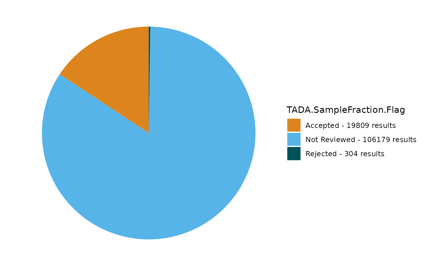
TADA_FieldValuesPie(dataset_flags, field = "TADA.MethodSpeciation.Flag")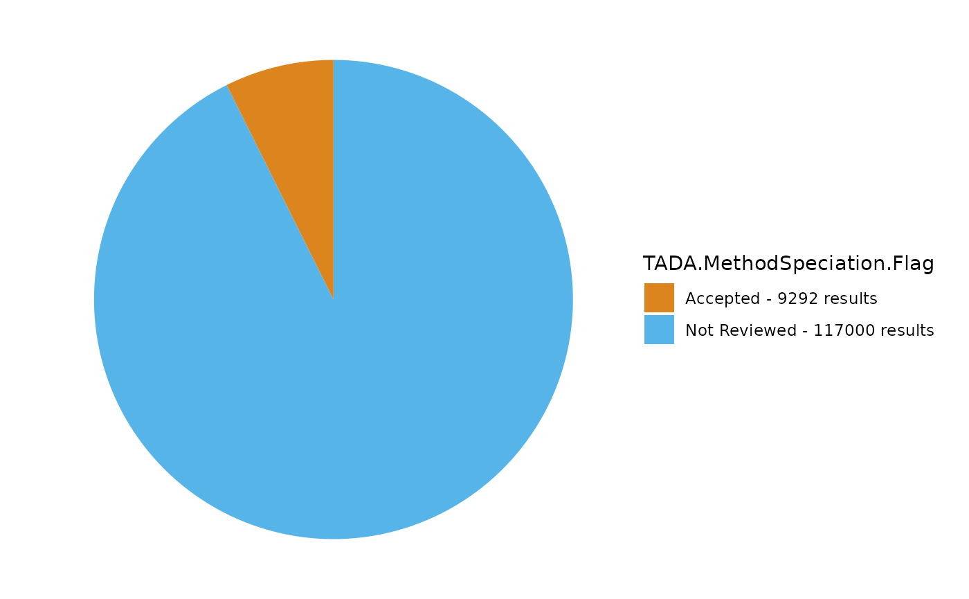
TADA_FieldValuesPie(dataset_flags, field = "TADA.ResultUnit.Flag")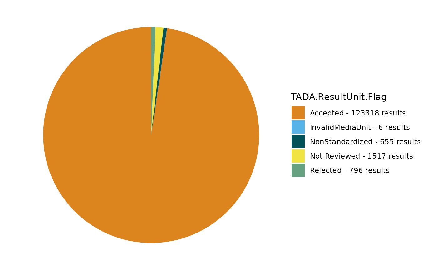
TADA_FieldValuesPie(dataset_flags, field = "TADA.ActivityType.Flag")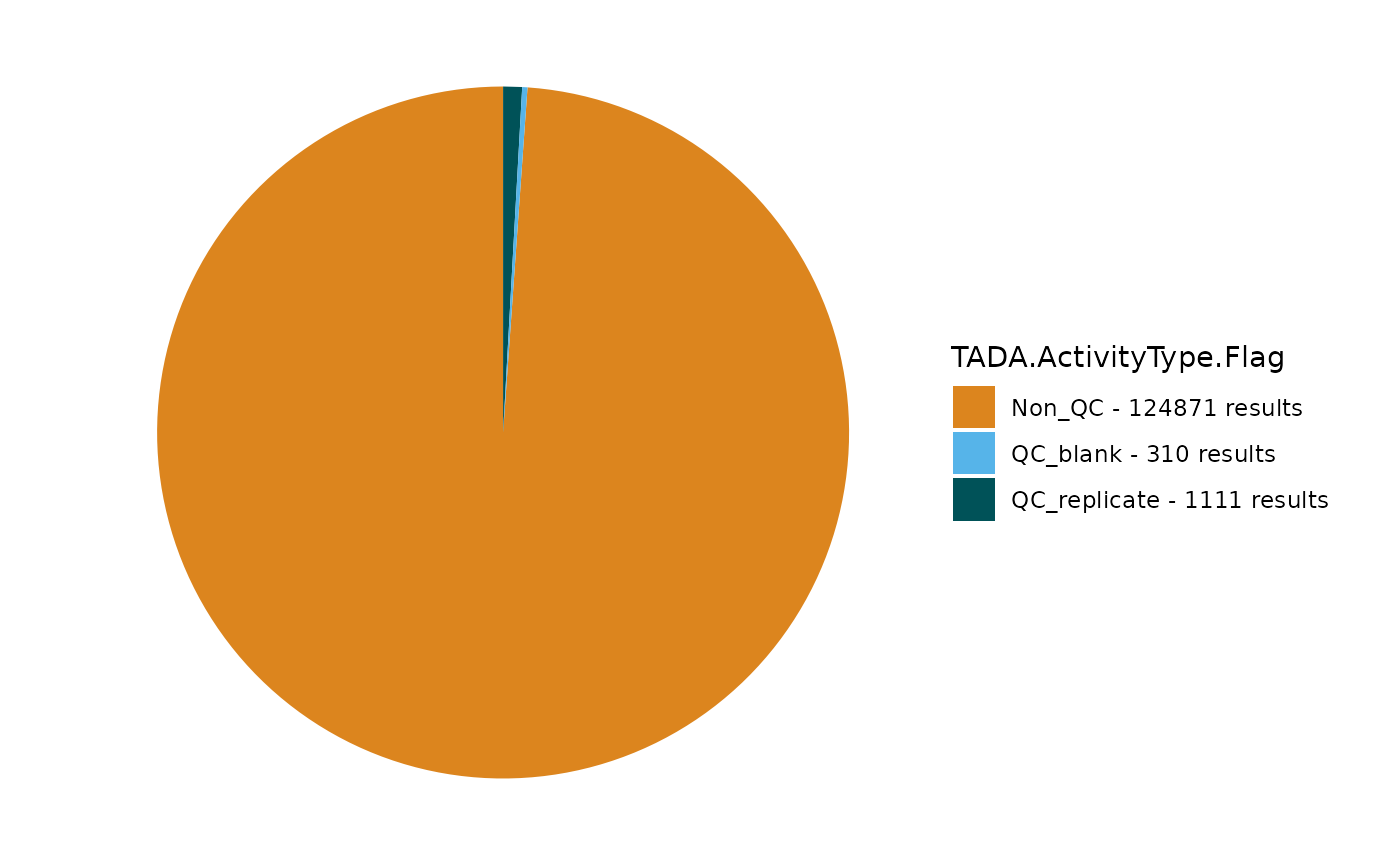
Any results flagged as “Suspect” are recognized in the QAQC Validation Table as having some data quality issue. “NonStandardized” means that the format has not been fully vetted or processed, while “Pass” confirms that the characteristic combination is widely recognized as correctly formatted. Let’s add any suspect results to the removed dataframe for later review.
Note: if you find any errors in the QAQC Validation Table, please contact the WQX Help Desk at WQX@epa.gov to help correct it. Thanks in advance!
# grab all the flagged results from the four functions
problem_flagged <- dataset_flags |>
dplyr::filter(TADA.SampleFraction.Flag == "Suspect" | TADA.MethodSpeciation.Flag == "Suspect" | TADA.ResultUnit.Flag == "Suspect" | !TADA.ActivityType.Flag %in% ("Non_QC")) |>
dplyr::mutate(TADA.RemovalReason = "Invalid Unit, Method, Speciation, or Activity Type.")
dataset_flags <- dataset_flags |> dplyr::filter(!ResultIdentifier %in% problem_flagged$ResultIdentifier)
# create dataframe of removed results
removed <- plyr::rbind.fill(removed, problem_flagged)
# remove df no longer needed
rm(problem_flagged)
# dimension check
dimCheck(all_result_num, dataset_flags, removed, checkName = "Filter Flag Functions")## [1] "Good to go. Zero results created or destroyed in Filter Flag Functions check."Question 7: Are there any other metadata columns that you review and filter in your workflow?
We’ve finished running the recommended flagging functions and removing results that do not pass QC checks. Let’s look at the breakdown of these data in the removed object.
removal <- TADA_FieldValuesTable(removed, field = "TADA.RemovalReason")
removal## Value
## 1 Invalid Unit, Method, Speciation, or Activity Type.
## 2 Result value type cannot be converted to numeric or no detection limit values provided.
## 3 Activity media is not water.
## 4 Detection limit information contains errors or missing information.
## Count
## 1 35809
## 2 13418
## 3 5050
## 4 18You can review any other columns of interest and create custom domain tables of your “Valid” and “Invalid” criteria using R or Excel. Also check out some of the other flagging functions available in TADA:
?TADA_FindNearbySites()?TADA_FindPotentialDuplicatesMultipleOrgs()?TADA_FindPotentialDuplicatesSingleOrg()?TADA_FindQAPPApproval()?TADA_FindQAPPDoc()?TADA_FlagAboveThreshold()?TADA_FlagBelowThreshold()?TADA_FlagContinuousData()?TADA_FlagCoordinates()?TADA_FlagMeasureQualifierCode()?TADA_FlagMethod()
Please let us know of other flagging functions you think would have broad appeal in the TADA package or need assistance brainstorming/developing.
Censored data handling
We have already identified, flagged, and in some cases removed problematic detection limit data from our dataframe, but that doesn’t keep them from being difficult. Because we do not know the result value with adequate precision, water quality data users often set non-detect values to some number below the reported detection limit. TADA contains some simple methods for handling detection limits: users may multiply the detection limit by some number between 0 and 1, or convert the detection limit value to a random number between 0 and the detection limit. More complex detection limit estimation requiring regression models (Maximum Likelihood, Kaplan-Meier, Robust Regression on Order Statistics) or similar must be performed outside of the current version of TADA (though future development is planned).
Question 8: How would you parameterize
TADA_SimpleCensoredMethods() to make non-detect values
equal to the provided detection limit? What would you need to change in
the example below?
dataset_cens <- TADA_SimpleCensoredMethods(dataset_flags,
nd_method = "multiplier",
nd_multiplier = 0.5,
od_method = "as-is"
)Let’s take a look at how the censored data handling function affects
the TADA.ResultMeasureValueDataTypes.Flag column.
First, we can look use TADA_FieldValuesTable to look at
the TADA.ResultMeasureValueDataTypes.Flag column in data set before we
ran TADA_SimpleCensoredMethods.
# before
TADA_FieldValuesTable(dataset_flags, field = "TADA.ResultMeasureValueDataTypes.Flag")## Value Count
## 1 Numeric 87532
## 2 Percentage 992
## 3 Numeric Range - Averaged 266
## 4 Less Than 18
## 5 Greater Than 9
## 6 Comma-Separated Numeric 7Then we can use TADA_FieldValuesTable again to look at
the same column after TADA_SimpleCensoredMethods.
# after
TADA_FieldValuesTable(dataset_cens, field = "TADA.ResultMeasureValueDataTypes.Flag")## Value Count
## 1 Numeric 87527
## 2 Percentage 992
## 3 Numeric Range - Averaged 266
## 4 Less Than 18
## 5 Greater Than 9
## 6 Comma-Separated Numeric 7
## 7 Result Value/Unit Estimated from Detection Limit 5Question 9: Is there a difference between the first and second tables?
If you’d like to start thinking about using statistical methods to
estimate detection limit values, check out the ?TADA_Stats
function, which accepts user-defined data groupings (or defaults to
TADA.ComparableDataIdentifier to determine measurement count, location
count, censored data stats, min, max, and percentile stats, and suggests
non-detect estimation methods based on the number of results, % of data
frame censored, and number of censoring levels (detection limits). The
decision tree used in the function was outlined in a National
Nonpoint Source Tech Memo.
Data exploration
How are you feeling about your test dataframe? Does it seem ready for
the next step(s) in your analyses? There’s probably a lot more you’d
like to look at/filter out before you’re ready to say: QC complete.
Let’s first check out characteristics in the dataframe using
dplyr functions and pipes.
# get table of characteristics with number of results, sites, and organizations
dataset_cens_summary <- dataset_cens |>
dplyr::group_by(TADA.CharacteristicName) |>
dplyr::summarise(Result_Count = length(ResultIdentifier), Site_Count = length(unique(TADA.MonitoringLocationIdentifier)), Org_Count = length(unique(OrganizationIdentifier))) |>
dplyr::arrange(desc(Result_Count))You may see a characteristic that you’d like to investigate further
in isolation. TADA_FieldValuesPie() will also produce
summary pie charts for a given column within a specific
characteristic. Let’s take a look.
# go ahead and pick a characteristic name from the table generated above. I picked dissolved oxygen (DO) amd selected OrganizationFormalName as the field to see the relative contribution of each org to DO results
TADA_FieldValuesPie(dataset_cens, field = "OrganizationFormalName", characteristicName = "DISSOLVED OXYGEN (DO)")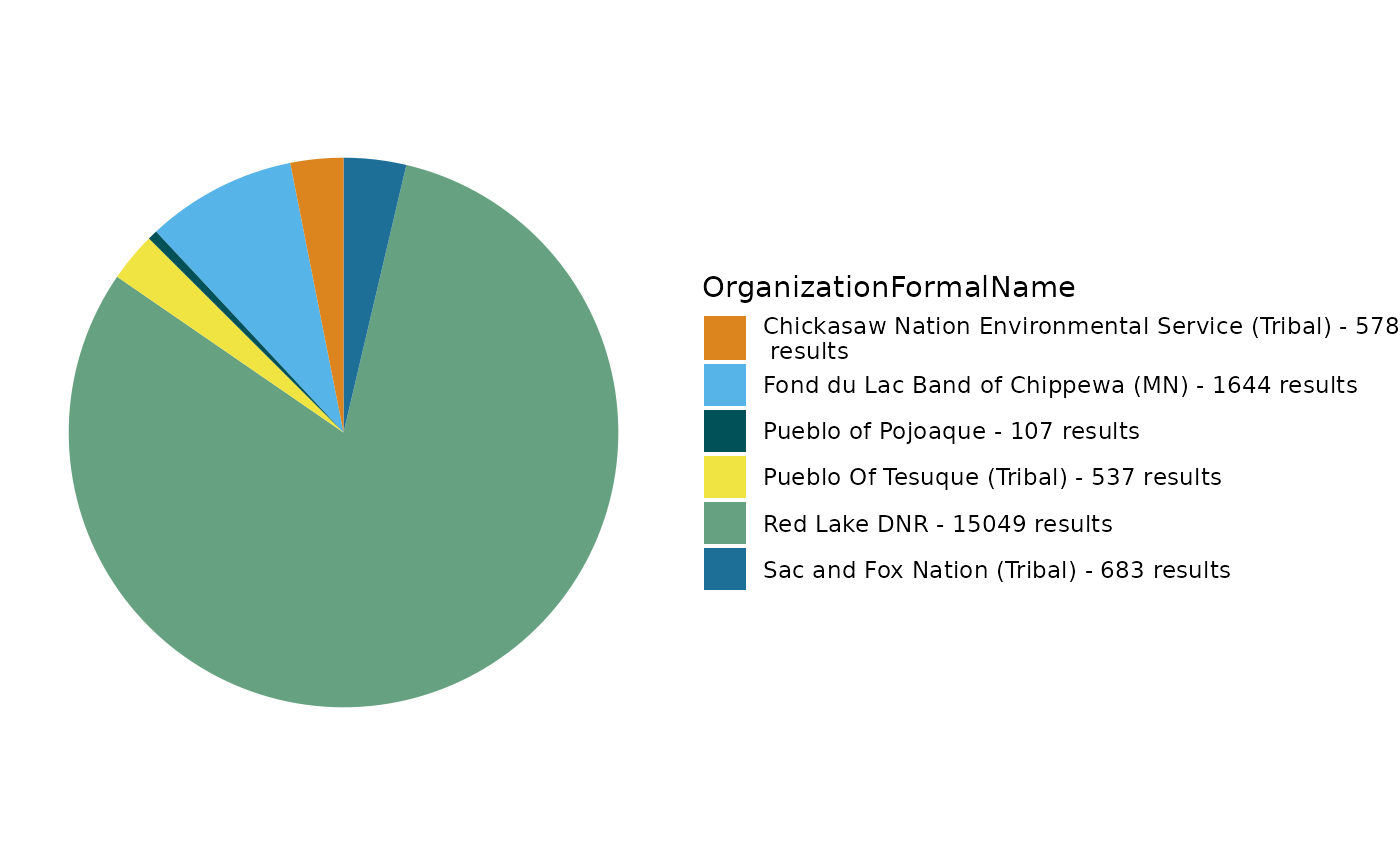
We can view the site locations using a TADA mapping function. In this map, the circles indicate monitoring locations in the data set; their size corresponds to the number of results collected at that site, while the darker the circle, the more characteristics were sampled at that site.
TADA_OverviewMap(dataset_cens)