Continuous Data
Table of Contents
Quickstart
To run a continuous dataset:
import pybmds

# create a continuous dataset
dataset = pybmds.ContinuousDataset(
    doses=[0, 25, 50, 75, 100],
    ns=[20, 20, 20, 20, 20],
    means=[6, 8, 13, 25, 30],
    stdevs=[4, 4.3, 3.8, 4.4, 3.7],
)

# create a session
session = pybmds.Session(dataset=dataset)
session.add_default_models()

# execute the session; recommend best-fitting model
session.execute_and_recommend()

# save excel report
df = session.to_df()
df.to_excel("output/report.xlsx")

# save to a word report
report = session.to_docx()
report.save("output/report.docx")
Continuous datasets
Continuous datasets can defined using group level summary data or individual response data.
A continuous summary dataset requires a list of doses, mean responses, standard deviations, and the total number of subjects. All lists must be the same size, and there should be one item in each list for each dose-group.
You can also add optional attributes, such as name, dose_name, dose_units, response_name, response_units, etc.
For example:
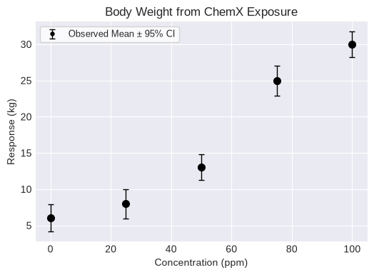
dataset = pybmds.ContinuousDataset(
    name="Body Weight from ChemX Exposure",
    dose_name="Concentration",
    dose_units="ppm",
    response_units="kg",
    doses=[0, 25, 50, 75, 100],
    ns=[20, 20, 20, 20, 20],
    means=[6, 8, 13, 25, 30],
    stdevs=[4, 4.3, 3.8, 4.4, 3.7],
)
fig = dataset.plot(figsize=(6,4))
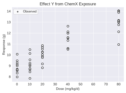
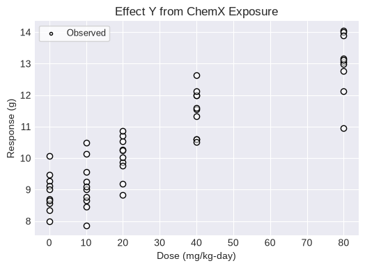
A continuous individual dataset requires the dose and response for each individual. Both lists must be the same size. Additional options can also be added such as the name or units:
dataset2 = pybmds.ContinuousIndividualDataset(
    name="Effect Y from ChemX Exposure",
    dose_name="Dose",
    dose_units="mg/kg/d",
    response_units="g",
    doses=[
            0, 0, 0, 0, 0, 0, 0, 0, 0, 0,
            10, 10, 10, 10, 10, 10, 10, 10, 10, 10,
            20, 20, 20, 20, 20, 20, 20, 20, 20, 20,
            40, 40, 40, 40, 40, 40, 40, 40, 40, 40,
            80, 80, 80, 80, 80, 80, 80, 80, 80, 80,
        ],
    responses=[
        8.57, 8.71, 7.99, 9.27, 9.47, 10.06, 8.65, 9.13, 9.01, 8.35,
        8.66, 8.45, 9.26, 8.76, 7.85, 9.01, 9.09, 9.57, 10.14, 10.49,
        9.87, 10.26, 9.76, 10.24, 10.54, 10.72, 8.83, 10.02, 9.18, 10.87,
        11.56, 10.59, 11.99, 11.59, 10.59, 10.52, 11.32, 12.0, 12.12, 12.64,
        10.96, 12.13, 12.77, 13.06, 13.16, 14.04, 14.01, 13.9, 12.99, 13.13,
    ],
)
fig = dataset2.plot(figsize=(6,4))
Single model fit
You can fit a specific model to the dataset and plot/print the results. The printed results will include the BMD, BMDL, BMDU, p-value, AIC, etc.
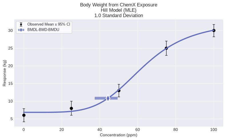
For example, to fit the Hill model, run the following code and plot the results:
from pybmds.models import continuous

model = continuous.Hill(dataset)
model.execute()
fig = model.plot()
To view an output report:
print(model.text())
          Hill Model
══════════════════════════════

Version: pybmds 25.2 (bmdscore 25.2)

Input Summary:
╒══════════════════════════════╤════════════════════════════╕
│ BMR                          │ 1.0 Standard Deviation     │
│ Distribution                 │ Normal + Constant variance │
│ Modeling Direction           │ Up (↑)                     │
│ Confidence Level (one sided) │ 0.95                       │
│ Modeling Approach            │ MLE                        │
╘══════════════════════════════╧════════════════════════════╛

Parameter Settings:
╒═════════════╤═══════════╤═══════╤═══════╕
│ Parameter   │   Initial │   Min │   Max │
╞═════════════╪═══════════╪═══════╪═══════╡
│ g           │         0 │  -100 │   100 │
│ v           │         0 │  -100 │   100 │
│ k           │         0 │     0 │     5 │
│ n           │         1 │     1 │    18 │
│ alpha       │         0 │   -18 │    18 │
╘═════════════╧═══════════╧═══════╧═══════╛

Modeling Summary:
╒════════════════╤═════════════╕
│ BMD            │   44.3603   │
│ BMDL           │   37.4378   │
│ BMDU           │   49.4299   │
│ AIC            │  570.3      │
│ Log-Likelihood │ -280.15     │
│ P-Value        │    0.163921 │
│ Model d.f.     │    1        │
╘════════════════╧═════════════╛

Model Parameters:
╒════════════╤════════════╤════════════╤═════════════╕
│ Variable   │   Estimate │ On Bound   │   Std Error │
╞════════════╪════════════╪════════════╪═════════════╡
│ g          │    6.80589 │ no         │    0.689269 │
│ v          │   25.6632  │ no         │    2.65373  │
│ k          │   62.7872  │ no         │    3.59334  │
│ n          │    4.87539 │ no         │    1.08357  │
│ alpha      │   15.881   │ no         │   35.6668   │
╘════════════╧════════════╧════════════╧═════════════╛

Goodness of Fit:
╒════════╤═════╤═══════════════╤═════════════════════╤═══════════════════╕
│   Dose │   N │   Sample Mean │   Model Fitted Mean │   Scaled Residual │
╞════════╪═════╪═══════════════╪═════════════════════╪═══════════════════╡
│      0 │  20 │             6 │             6.80589 │        -0.904381  │
│     25 │  20 │             8 │             7.09076 │         1.02037   │
│     50 │  20 │            13 │            13.1658  │        -0.186064  │
│     75 │  20 │            25 │            24.8734  │         0.14202   │
│    100 │  20 │            30 │            30.0641  │        -0.0719426 │
╘════════╧═════╧═══════════════╧═════════════════════╧═══════════════════╛
╒════════╤═════╤═════════════╤═══════════════════╕
│   Dose │   N │   Sample SD │   Model Fitted SD │
╞════════╪═════╪═════════════╪═══════════════════╡
│      0 │  20 │         4   │           3.98509 │
│     25 │  20 │         4.3 │           3.98509 │
│     50 │  20 │         3.8 │           3.98509 │
│     75 │  20 │         4.4 │           3.98509 │
│    100 │  20 │         3.7 │           3.98509 │
╘════════╧═════╧═════════════╧═══════════════════╛

Likelihoods:
╒═════════╤══════════════════╤════════════╤═════════╕
│ Model   │   Log-Likelihood │   # Params │     AIC │
╞═════════╪══════════════════╪════════════╪═════════╡
│ A1      │         -279.181 │          6 │ 570.362 │
│ A2      │         -278.726 │         10 │ 577.452 │
│ A3      │         -279.181 │          6 │ 570.362 │
│ fitted  │         -280.15  │          5 │ 570.3   │
│ reduced │         -374.79  │          2 │ 753.579 │
╘═════════╧══════════════════╧════════════╧═════════╛

Tests of Mean and Variance Fits:
╒════════╤══════════════════════════════╤═════════════╤═══════════╕
│ Name   │   -2 * Log(Likelihood Ratio) │   Test d.f. │   P-Value │
╞════════╪══════════════════════════════╪═════════════╪═══════════╡
│ Test 1 │                   192.127    │           8 │  0        │
│ Test 2 │                     0.909828 │           4 │  0.923147 │
│ Test 3 │                     0.909828 │           4 │  0.923147 │
│ Test 4 │                     1.93767  │           1 │  0.163921 │
╘════════╧══════════════════════════════╧═════════════╧═══════════╛
Test 1: Test the null hypothesis that responses and variances don't differ among dose levels
(A2 vs R).  If this test fails to reject the null hypothesis (p-value > 0.05), there may not be
a dose-response.

Test 2: Test the null hypothesis that variances are homogenous (A1 vs A2).  If this test fails to
reject the null hypothesis (p-value > 0.05), the simpler constant variance model may be appropriate.

Test 3: Test the null hypothesis that the variances are adequately modeled (A3 vs A2). If this test
fails to reject the null hypothesis (p-value > 0.05), it may be inferred that the variances have
been modeled appropriately.

Test 4: Test the null hypothesis that the model for the mean fits the data (Fitted vs A3). If this
test fails to reject the null hypothesis (p-value > 0.1), the user has support for use of the
selected model.
You can change the range and initial value for any parameter in the model by following the same steps above.
Change input settings
The default settings when running a continuous analysis are a BMR of 1 standard deviation from the BMD, a 95% confidence interval, and a normally distributed and constant variance between dose groups.
If you fit a single model to your dataset, you can change these settings:
model = continuous.Hill(dataset)
print(model.settings.tbl())
print(model.priors_tbl())
╒══════════════════════════════╤════════════════════════════╕
│ BMR                          │ 1.0 Standard Deviation     │
│ Distribution                 │ Normal + Constant variance │
│ Modeling Direction           │ Up (↑)                     │
│ Confidence Level (one sided) │ 0.95                       │
│ Modeling Approach            │ MLE                        │
│ Degree                       │ 0                          │
╘══════════════════════════════╧════════════════════════════╛
╒═════════════╤═══════════╤═══════╤═══════╕
│ Parameter   │   Initial │   Min │   Max │
╞═════════════╪═══════════╪═══════╪═══════╡
│ g           │         0 │  -100 │   100 │
│ v           │         0 │  -100 │   100 │
│ k           │         0 │     0 │     5 │
│ n           │         1 │     1 │    18 │
│ alpha       │         0 │   -18 │    18 │
╘═════════════╧═══════════╧═══════╧═══════╛
You can change individual model settings:
model = continuous.Hill(
    dataset,
    settings={
        "bmr": 0.1,
        "bmr_type": pybmds.ContinuousRiskType.RelativeDeviation,
        "disttype": pybmds.ContinuousDistType.normal_ncv,
    },
)
model.settings.priors.update("k", max_value=3)
print(model.settings.tbl())
print(model.priors_tbl())
╒══════════════════════════════╤═══════════════════════════════╕
│ BMR                          │ 10% Relative Deviation        │
│ Distribution                 │ Normal + Nonconstant variance │
│ Modeling Direction           │ Up (↑)                        │
│ Confidence Level (one sided) │ 0.95                          │
│ Modeling Approach            │ MLE                           │
│ Degree                       │ 0                             │
╘══════════════════════════════╧═══════════════════════════════╛
╒═════════════╤═══════════╤═══════╤═══════╕
│ Parameter   │   Initial │   Min │   Max │
╞═════════════╪═══════════╪═══════╪═══════╡
│ g           │         0 │  -100 │   100 │
│ v           │         0 │  -100 │   100 │
│ k           │         0 │     0 │     3 │
│ n           │         1 │     1 │    18 │
│ rho         │         0 │   -18 │    18 │
│ alpha       │         0 │   -18 │    18 │
╘═════════════╧═══════════╧═══════╧═══════╛
For the Polynomial model, degrees can be increased to a maximum of the lesser of n-1 or 8, where n is the number of dose groups.
continuous.Polynomial(dataset, settings={"degree": 2})
continuous.Polynomial(dataset, settings={"degree": 3})
<pybmds.models.continuous.Polynomial at 0x7fba9121f6f0>
Change parameter settings
To see a preview of the initial parameter settings:
model = continuous.Hill(dataset)
print(model.settings.tbl())
print(model.priors_tbl())
╒══════════════════════════════╤════════════════════════════╕
│ BMR                          │ 1.0 Standard Deviation     │
│ Distribution                 │ Normal + Constant variance │
│ Modeling Direction           │ Up (↑)                     │
│ Confidence Level (one sided) │ 0.95                       │
│ Modeling Approach            │ MLE                        │
│ Degree                       │ 0                          │
╘══════════════════════════════╧════════════════════════════╛
╒═════════════╤═══════════╤═══════╤═══════╕
│ Parameter   │   Initial │   Min │   Max │
╞═════════════╪═══════════╪═══════╪═══════╡
│ g           │         0 │  -100 │   100 │
│ v           │         0 │  -100 │   100 │
│ k           │         0 │     0 │     5 │
│ n           │         1 │     1 │    18 │
│ alpha       │         0 │   -18 │    18 │
╘═════════════╧═══════════╧═══════╧═══════╛
You can also change the initial parameter settings shown above for any run of a single continuous model. Continuing with the Hill model example, you can set the power parameter n to be equal to 1. You do this by changing the initial, minimum, and maximum values of that parameter:
model = continuous.Hill(dataset)
model.settings.priors.update("n", initial_value=1, min_value=1, max_value=1)
print(model.priors_tbl())
╒═════════════╤═══════════╤═══════╤═══════╕
│ Parameter   │   Initial │   Min │   Max │
╞═════════════╪═══════════╪═══════╪═══════╡
│ g           │         0 │  -100 │   100 │
│ v           │         0 │  -100 │   100 │
│ k           │         0 │     0 │     5 │
│ n           │         1 │     1 │     1 │
│ alpha       │         0 │   -18 │    18 │
╘═════════════╧═══════════╧═══════╧═══════╛
Multiple model fit (sessions) and model recommendation
To run all the default models, save the results, and save the plot of the fit of the recommended model with the data:
# create a continuous dataset
dataset = pybmds.ContinuousDataset(
doses=[0, 25, 50, 75, 100],
ns=[20, 20, 20, 20, 20],
means=[6, 8, 13, 25, 30],
stdevs=[4, 4.3, 3.8, 4.4, 3.7],
)
session = pybmds.Session(dataset=dataset)
session.add_default_models()
# execute the session
session.execute()
# recommend a best-fitting model
session.recommend()
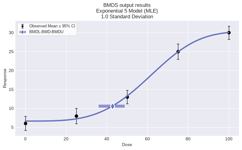
# print recommended model and plot recommended model with dataset
model_index = session.recommender.results.recommended_model_index
if model_index:
model = session.models[model_index]
fig = model.plot()
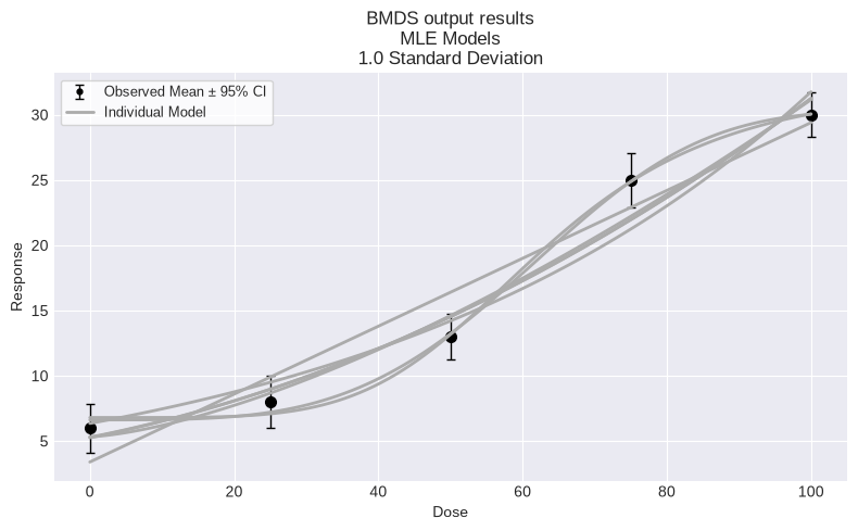
You can also plot all models:
fig = session.plot()
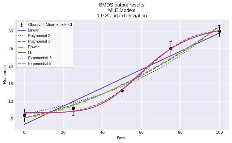
fig = session.plot(colorize=False)
To print a summary table of modeling results, create a custom function:
import pandas as pd

def summary_table(session):
    data = []
    for model in session.models:
        data.append([
            model.name(),
            model.results.bmdl,
            model.results.bmd,
            model.results.bmdu,
            model.results.tests.p_values[1],
            model.results.tests.p_values[2],
            model.results.tests.p_values[3],
            model.results.fit.aic
        ])

    df = pd.DataFrame(
        data=data,
        columns=["Model", "BMDL", "BMD", "BMDU", "P-Value 2", "P-Value 3", "P-Value 4", "AIC"]
    )
    return df

summary_table(session)
| Model | BMDL | BMD | BMDU | P-Value 2 | P-Value 3 | P-Value 4 | AIC | |
|---|---|---|---|---|---|---|---|---|
| 0 | Linear | 15.366633 | 17.590090 | 20.476330 | 0.923147 | 0.923147 | 0.000002 | 593.840104 |
| 1 | Polynomial 2 | 21.259623 | 28.096820 | 37.150471 | 0.923147 | 0.923147 | 0.000183 | 583.575133 |
| 2 | Polynomial 3 | 21.251732 | 28.285377 | 37.143031 | 0.923147 | 0.923147 | 0.000183 | 583.577496 |
| 3 | Power | 23.273696 | 29.484932 | 36.666906 | 0.923147 | 0.923147 | 0.000567 | 581.313910 |
| 4 | Hill | 37.437820 | 44.360266 | 49.429919 | 0.923147 | 0.923147 | 0.163921 | 570.299792 |
| 5 | Exponential 3 | 30.113771 | 33.000669 | 37.536866 | 0.923147 | 0.923147 | 0.000082 | 588.296076 |
| 6 | Exponential 5 | 36.037483 | 42.818144 | 48.801014 | 0.923147 | 0.923147 | 0.240277 | 569.741084 |
Change model settings
To change model settings to all default models added to a session:
session = pybmds.Session(dataset=dataset)
session.add_default_models(
    settings={
        "disttype": pybmds.ContinuousDistType.normal_ncv,
        "bmr_type": pybmds.ContinuousRiskType.AbsoluteDeviation,
        "bmr": 2,
        "alpha": 0.1,
    }
)
Run subset of models and select best fit
You can select a set of models and find the best fit, rather than using all of the default continuous models.
For example, to model average on the Hill, Linear, and Exponential 3:
session = pybmds.Session(dataset=dataset)
session.add_model(pybmds.Models.Linear)
session.add_model(pybmds.Models.ExponentialM3)
session.add_model(pybmds.Models.Hill)

session.execute()
Model recommendation and selection
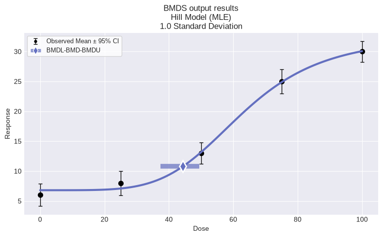
The pybmds package may recommend a best-fitting model based on a decision tree, but expert judgment may be required for model selection. To run model recommendation and view a recommended model, if one is recommended:
session.recommend()

if session.recommended_model is not None:
    display(session.recommended_model.plot())
    print(session.recommended_model.text())
          Hill Model
══════════════════════════════

Version: pybmds 25.2 (bmdscore 25.2)

Input Summary:
╒══════════════════════════════╤════════════════════════════╕
│ BMR                          │ 1.0 Standard Deviation     │
│ Distribution                 │ Normal + Constant variance │
│ Modeling Direction           │ Up (↑)                     │
│ Confidence Level (one sided) │ 0.95                       │
│ Modeling Approach            │ MLE                        │
╘══════════════════════════════╧════════════════════════════╛

Parameter Settings:
╒═════════════╤═══════════╤═══════╤═══════╕
│ Parameter   │   Initial │   Min │   Max │
╞═════════════╪═══════════╪═══════╪═══════╡
│ g           │         0 │  -100 │   100 │
│ v           │         0 │  -100 │   100 │
│ k           │         0 │     0 │     5 │
│ n           │         1 │     1 │    18 │
│ alpha       │         0 │   -18 │    18 │
╘═════════════╧═══════════╧═══════╧═══════╛

Modeling Summary:
╒════════════════╤═════════════╕
│ BMD            │   44.3603   │
│ BMDL           │   37.4378   │
│ BMDU           │   49.4299   │
│ AIC            │  570.3      │
│ Log-Likelihood │ -280.15     │
│ P-Value        │    0.163921 │
│ Model d.f.     │    1        │
╘════════════════╧═════════════╛

Model Parameters:
╒════════════╤════════════╤════════════╤═════════════╕
│ Variable   │   Estimate │ On Bound   │   Std Error │
╞════════════╪════════════╪════════════╪═════════════╡
│ g          │    6.80589 │ no         │    0.689269 │
│ v          │   25.6632  │ no         │    2.65373  │
│ k          │   62.7872  │ no         │    3.59334  │
│ n          │    4.87539 │ no         │    1.08357  │
│ alpha      │   15.881   │ no         │   35.6668   │
╘════════════╧════════════╧════════════╧═════════════╛

Goodness of Fit:
╒════════╤═════╤═══════════════╤═════════════════════╤═══════════════════╕
│   Dose │   N │   Sample Mean │   Model Fitted Mean │   Scaled Residual │
╞════════╪═════╪═══════════════╪═════════════════════╪═══════════════════╡
│      0 │  20 │             6 │             6.80589 │        -0.904381  │
│     25 │  20 │             8 │             7.09076 │         1.02037   │
│     50 │  20 │            13 │            13.1658  │        -0.186064  │
│     75 │  20 │            25 │            24.8734  │         0.14202   │
│    100 │  20 │            30 │            30.0641  │        -0.0719426 │
╘════════╧═════╧═══════════════╧═════════════════════╧═══════════════════╛
╒════════╤═════╤═════════════╤═══════════════════╕
│   Dose │   N │   Sample SD │   Model Fitted SD │
╞════════╪═════╪═════════════╪═══════════════════╡
│      0 │  20 │         4   │           3.98509 │
│     25 │  20 │         4.3 │           3.98509 │
│     50 │  20 │         3.8 │           3.98509 │
│     75 │  20 │         4.4 │           3.98509 │
│    100 │  20 │         3.7 │           3.98509 │
╘════════╧═════╧═════════════╧═══════════════════╛

Likelihoods:
╒═════════╤══════════════════╤════════════╤═════════╕
│ Model   │   Log-Likelihood │   # Params │     AIC │
╞═════════╪══════════════════╪════════════╪═════════╡
│ A1      │         -279.181 │          6 │ 570.362 │
│ A2      │         -278.726 │         10 │ 577.452 │
│ A3      │         -279.181 │          6 │ 570.362 │
│ fitted  │         -280.15  │          5 │ 570.3   │
│ reduced │         -374.79  │          2 │ 753.579 │
╘═════════╧══════════════════╧════════════╧═════════╛

Tests of Mean and Variance Fits:
╒════════╤══════════════════════════════╤═════════════╤═══════════╕
│ Name   │   -2 * Log(Likelihood Ratio) │   Test d.f. │   P-Value │
╞════════╪══════════════════════════════╪═════════════╪═══════════╡
│ Test 1 │                   192.127    │           8 │  0        │
│ Test 2 │                     0.909828 │           4 │  0.923147 │
│ Test 3 │                     0.909828 │           4 │  0.923147 │
│ Test 4 │                     1.93767  │           1 │  0.163921 │
╘════════╧══════════════════════════════╧═════════════╧═══════════╛
Test 1: Test the null hypothesis that responses and variances don't differ among dose levels
(A2 vs R).  If this test fails to reject the null hypothesis (p-value > 0.05), there may not be
a dose-response.

Test 2: Test the null hypothesis that variances are homogenous (A1 vs A2).  If this test fails to
reject the null hypothesis (p-value > 0.05), the simpler constant variance model may be appropriate.

Test 3: Test the null hypothesis that the variances are adequately modeled (A3 vs A2). If this test
fails to reject the null hypothesis (p-value > 0.05), it may be inferred that the variances have
been modeled appropriately.

Test 4: Test the null hypothesis that the model for the mean fits the data (Fitted vs A3). If this
test fails to reject the null hypothesis (p-value > 0.1), the user has support for use of the
selected model.
You can select a best-fitting model and output reports generated will indicate this selection. This is a manual action. The example below selects the recommended model, but any model in the session could be selected.
session.select(model=session.recommended_model, notes="Lowest AIC; recommended model")
Changing how parameters are counted
For the purposes of statistical calculations, e.g., calcuation the AIC value and p-values, BMDS only counts the number of parameters off their respective boundaries by default. But users have the option of parameterizing BMDS so that it counts all the parameters in a model, irrespective if they were estimated on or off of their boundaries.
Parameterizing BMDS to count all parameters will impact AIC and p-value calculations and therefore may impact the selection of models using the automatic model selection logic. For example, consider the following dataset run using the default setting of only counting parameters that are off a boundary.
import pybmds
import pandas as pd

dataset = pybmds.ContinuousDataset(
    doses=[0, 25, 50, 100, 200],
    ns=[20, 20, 20, 20, 20],
    means=[6.1, 6.3, 9.5, 15.2, 30.1],
    stdevs=[3.5, 3.3, 4.1, 3.6, 4.5],
)

# create a BMD session
session = pybmds.Session(dataset=dataset)

# add all default models
session.add_default_models()

# execute the session
session.execute()

# recommend a best-fitting model
session.recommend()

# # Print out a summary table for the recommended model

model = session.recommended_model
if model is not None:
    df = pd.DataFrame([[
        model.name(),
        model.results.bmdl,
        model.results.bmd,
        model.results.bmdu,
        model.results.tests.dfs[3],
        model.results.tests.p_values[1],
        model.results.tests.p_values[2],
        model.results.tests.p_values[3],
        model.results.fit.aic
    ]], columns=["Model", "BMDL", "BMD", "BMDU", "DF", "P-Value 2", "P-Value 3", "P-Value 4", "AIC"])
    df = df.T  # Transpose for vertical display
    df.columns = ["Value"]
    display(df)

else:
    print("No recommended model.")

fig = session.recommended_model.plot()
| Value | |
|---|---|
| Model | Power |
| BMDL | 39.398522 |
| BMD | 51.656812 |
| BMDU | 66.659426 |
| DF | 2.0 |
| P-Value 2 | 0.62439 |
| P-Value 3 | 0.62439 |
| P-Value 4 | 0.554879 |
| AIC | 556.15748 |
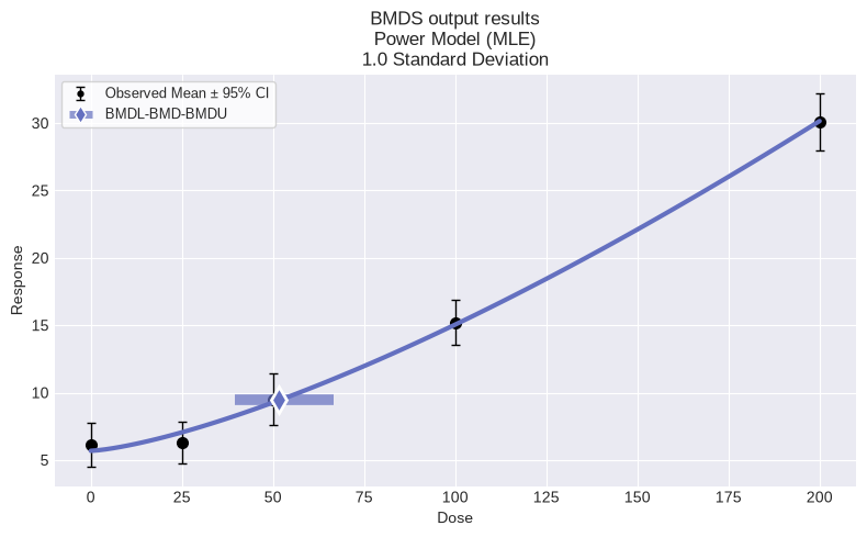
So, for this dataset, we can see that the automated model selection workflow chose the Power model. We can also summarize the modeling results for all models in the session by using the summary_table function defined above:
summary_table(session)
| Model | BMDL | BMD | BMDU | P-Value 2 | P-Value 3 | P-Value 4 | AIC | |
|---|---|---|---|---|---|---|---|---|
| 0 | Linear | 27.666465 | 31.528232 | 36.478962 | 0.62439 | 0.62439 | 0.008986 | 564.555495 |
| 1 | Polynomial 2 | 36.344045 | 48.525378 | 65.479921 | 0.62439 | 0.62439 | 0.356536 | 557.042107 |
| 2 | Polynomial 3 | 35.291785 | 47.083971 | 48.058609 | 0.62439 | 0.62439 | 0.337252 | 557.153318 |
| 3 | Power | 39.398522 | 51.656812 | 66.659426 | 0.62439 | 0.62439 | 0.554879 | 556.157480 |
| 4 | Hill | 41.381979 | 55.124484 | 72.138850 | 0.62439 | 0.62439 | 0.350988 | 557.849350 |
| 5 | Exponential 3 | 54.863034 | 60.386583 | 70.355170 | 0.62439 | 0.62439 | 0.142384 | 558.417644 |
| 6 | Exponential 5 | 40.393539 | 55.053391 | 72.461275 | 0.62439 | 0.62439 | 0.347962 | 557.860344 |
Further, we can also define a custom function to print out a table of models that had at least one parameter estimated on a bound:
def summary_parameter_bounds_table(session):
    rows = []
    for model in session.models:
        params = model.results.parameters
        for name, value, bounded in zip(params.names, params.values, params.bounded):
            if bool(bounded):
                rows.append({
                    "Model": model.name(),
                    "Parameter": name,
                    "Value": value,
                    "On Bound": bool(bounded)
            })
    df = pd.DataFrame(rows)
    display(df)

# Usage:
summary_parameter_bounds_table(session)
| Model | Parameter | Value | On Bound | |
|---|---|---|---|---|
| 0 | Polynomial 3 | b3 | 1.211492e-07 | True |
| 1 | Exponential 3 | d | 1.000000e+00 | True |
We can see above that only two models, the Polynomial 3 and Exponential 3, had parameters estimated on a bound. So, although it seems like the issue of parameters not being counted for AIC or p-value calculation when on a boundary, we can can re-model this dataset parameterizing BMDS to count all parameters in a model to to confirm whether that assumption is accurate:
session2 = pybmds.Session(dataset=dataset)
session2.add_default_models(
    settings={
        "count_all_parameters_on_boundary": True
    }
)
session2.execute()

# recommend a best-fitting model
session2.recommend()

# Print out a summary table for the recommended model
model = session2.recommended_model
if model is not None:
    df2 = pd.DataFrame([[
        model.name(),
        model.results.bmdl,
        model.results.bmd,
        model.results.bmdu,
        model.results.tests.dfs[3],
        model.results.tests.p_values[1],
        model.results.tests.p_values[2],
        model.results.tests.p_values[3],
        model.results.fit.aic
    ]], columns=["Model", "BMDL", "BMD", "BMDU", "DF", "P-Value 2", "P-Value 3", "P-Value 4", "AIC"])
    df2 = df2.T  # Transpose for vertical display
    df2.columns = ["Value"]
    display(df2)

else:
    print("No recommended model.")

fig = session2.recommended_model.plot()
| Value | |
|---|---|
| Model | Power |
| BMDL | 39.398522 |
| BMD | 51.656812 |
| BMDU | 66.659426 |
| DF | 2.0 |
| P-Value 2 | 0.62439 |
| P-Value 3 | 0.62439 |
| P-Value 4 | 0.554879 |
| AIC | 556.15748 |
The Power model was still selected as the best fitting model, even when counting all parameters on a boundary. Printing out a summary table that compares the p-values and AICs for session and session2lets us examine why:
def compare_pvalue_aic(session_a, session_b):
    rows = []
    for model_a, model_b in zip(session_a.models, session_b.models):
        rows.append({
            "Model": model_a.name(),
            "Session P-Value": model_a.results.tests.p_values[3],
            "Session AIC": model_a.results.fit.aic,
            "Session2 P-Value": model_b.results.tests.p_values[3],
            "Session2 AIC": model_b.results.fit.aic,
        })
    df = pd.DataFrame(rows)
    display(df)

# Usage:
compare_pvalue_aic(session, session2)
| Model | Session P-Value | Session AIC | Session2 P-Value | Session2 AIC | |
|---|---|---|---|---|---|
| 0 | Linear | 0.008986 | 564.555495 | 0.008986 | 564.555495 |
| 1 | Polynomial 2 | 0.356536 | 557.042107 | 0.356536 | 557.042107 |
| 2 | Polynomial 3 | 0.337252 | 557.153318 | 0.140374 | 559.153318 |
| 3 | Power | 0.554879 | 556.157480 | 0.554879 | 556.157480 |
| 4 | Hill | 0.350988 | 557.849350 | 0.350988 | 557.849350 |
| 5 | Exponential 3 | 0.142384 | 558.417644 | 0.065935 | 560.417644 |
| 6 | Exponential 5 | 0.347962 | 557.860344 | 0.347962 | 557.860344 |
We can see that for the models that have parameters on a boundary (as reported above: Polynomial 3 and Exponential 3), the session2 AICs are higher than the session AICs due to more parameters being counted for the penalization term. The p-values for those models are also lower given the decrease in the degrees of freedom. Hence, because neither of these models were selected previously, the ultimate model selection results were not different between thesession2 and session analyses.
Jonckheere-Terpstra Trend Test
Individual Response Data
To test for a trend in a continuous dataset with responses measured in individuals using the Jonckheere-Terpstra trend test, first load an individual response continuous dataset. Note that this individual response dataset has an apparent strong increasing trend and the Jonckheere-Terpstra test will provided results that support or refute that observation.
dataset1 = pybmds.ContinuousIndividualDataset(
    name="Effect Y from ChemX Exposure",
    dose_name="Dose",
    dose_units="mg/kg-day",
    response_units="g",
    doses=[0, 0, 0, 0, 0, 0, 0, 0, 0, 0,
            10, 10, 10, 10, 10, 10, 10, 10, 10, 10,
            20, 20, 20, 20, 20, 20, 20, 20, 20, 20,
            40, 40, 40, 40, 40, 40, 40, 40, 40, 40,
            80, 80, 80, 80, 80, 80, 80, 80, 80, 80,
        ],
    responses=[
        8.57, 8.71, 7.99, 9.27, 9.47, 10.06, 8.65, 9.13, 9.01, 8.35,
        8.66, 8.45, 9.26, 8.76, 7.85, 9.01, 9.09, 9.57, 10.14, 10.49,
        9.87, 10.26, 9.76, 10.24, 10.54, 10.72, 8.83, 10.02, 9.18, 10.87,
        11.56, 10.59, 11.99, 11.59, 10.59, 10.52, 11.32, 12.0, 12.12, 12.64,
        10.96, 12.13, 12.77, 13.06, 13.16, 14.04, 14.01, 13.9, 12.99, 13.13,
    ],
)

fig = dataset1.plot(figsize=(6,4))
# Run the Jonckheere-Terpstra trend test for an increasing trend
#Note that dataset.trend will use the Jonckheere-Terpstra trend test given
# that the dataset is continuous.
result1 = dataset1.trend(hypothesis="increasing")

# Display the results for the increasing trend test
# The alternative hypothesis for the increasting trend test is that there is a monotonic increasing trend in the data.
print("Jonckheere-Terpstra Trend Test Result:")
print(result1.tbl())

# Run the two-sided test
# The alternative hypothesis for the two-sided trend test is that there is a monotonic trend in the data, either increasing or decreasing.
result1_two_sided = dataset1.trend(hypothesis="two-sided")

# Display the results for the two-sided trend test
print("Jonckheere-Terpstra Trend Test Result:")
print(result1_two_sided.tbl())
Jonckheere-Terpstra Trend Test Result:
╒════════════════════╤═══════════════════════╕
│ Hypothesis         │ increasing            │
│ Statistic          │ 914.0                 │
│ Approach (P-Value) │ approximate           │
│ P-Value            │ 7.068789997788372e-13 │
╘════════════════════╧═══════════════════════╛
Jonckheere-Terpstra Trend Test Result:
╒════════════════════╤════════════════════════╕
│ Hypothesis         │ two-sided              │
│ Statistic          │ 914.0                  │
│ Approach (P-Value) │ approximate            │
│ P-Value            │ 1.4137579995576743e-12 │
╘════════════════════╧════════════════════════╛
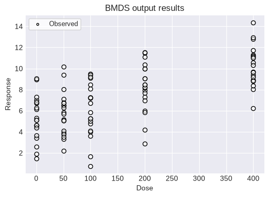
Alternatively, you can load an individual continuous response dataset from a CSV file and run the Jonckheere test on that data.
# Load the CSV file (make sure JT_strong_trend.csv is in the same directory)
df = pd.read_csv('data/JT_strong_trend.csv')

dataset2 = pybmds.ContinuousIndividualDataset(
    doses=df['doses'].values,
    responses=df['responses'].values,
)

fig = dataset2.plot(figsize=(6,4))
# Run the Jonckheere-Terpstra trend test for an increasing trend
result2 = dataset2.trend(hypothesis="increasing")

# Display the results for the increasing trend test
print("Jonckheere-Terpstra Trend Test Result:")
print(result2.tbl())

# Run the two-sided test
result2_two_sided = dataset2.trend(hypothesis="two-sided")

# Display the results for the two-sided trend test
print("Jonckheere-Terpstra Trend Test Result:")
print(result2_two_sided.tbl())
Jonckheere-Terpstra Trend Test Result:
╒════════════════════╤════════════════════════╕
│ Hypothesis         │ increasing             │
│ Statistic          │ 3065.0                 │
│ Approach (P-Value) │ approximate            │
│ P-Value            │ 4.5442649643234745e-11 │
╘════════════════════╧════════════════════════╛
Jonckheere-Terpstra Trend Test Result:
╒════════════════════╤═══════════════════════╕
│ Hypothesis         │ two-sided             │
│ Statistic          │ 3065.0                │
│ Approach (P-Value) │ approximate           │
│ P-Value            │ 9.088529928646949e-11 │
╘════════════════════╧═══════════════════════╛
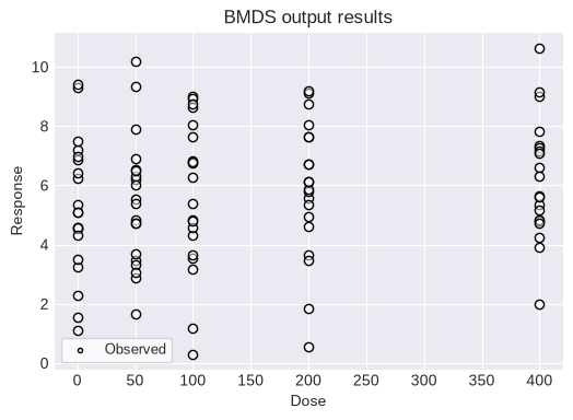
As a further example, the Jonckheere test can be run on a dataset with no apparent trend:
df2 = pd.read_csv('data/JT_no_trend.csv')

dataset3 = pybmds.ContinuousIndividualDataset(
    doses=df2['doses'].values,
    responses=df2['responses'].values,
)

fig = dataset3.plot(figsize=(6,4))
# Run the Jonckheere-Terpstra trend test for an increasing trend
result3 = dataset3.trend(hypothesis="increasing")

# Display the results for the increasing trend test
print("Jonckheere-Terpstra Trend Test Result:")
print(result3.tbl())

# Run the two-sided test
result3_two_sided = dataset3.trend(hypothesis="two-sided")

# Display the results for the two-sided trend test
print("Jonckheere-Terpstra Trend Test Result:")
print(result3_two_sided.tbl())
Jonckheere-Terpstra Trend Test Result:
╒════════════════════╤════════════════════╕
│ Hypothesis         │ increasing         │
│ Statistic          │ 2250.0             │
│ Approach (P-Value) │ approximate        │
│ P-Value            │ 0.0640732806328399 │
╘════════════════════╧════════════════════╛
Jonckheere-Terpstra Trend Test Result:
╒════════════════════╤════════════════════╕
│ Hypothesis         │ two-sided          │
│ Statistic          │ 2250.0             │
│ Approach (P-Value) │ approximate        │
│ P-Value            │ 0.1281465612656798 │
╘════════════════════╧════════════════════╛
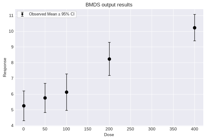
Summary Response Data
Often, only summary continuous data (reported as means and standard deviations) is available to risk assessors. The Jockheere-Terpstra trend test can stil be applied to such data after synthetic individual response data is generated. First, load and plot a summary dataset:
dataset4 = pybmds.ContinuousDataset(
    doses=[0, 50, 100, 200, 400],
    ns=[20, 20, 20, 20, 20],
    means=[5.26, 5.76, 6.13, 8.24, 10.23],
    stdevs=[2.03, 1.97, 2.47, 2.24, 1.8],
)
fig = dataset4.plot()
To run the Jonckheere-Terpstra trend test on the summary data, first, “synthetic” individual responses must be generated. These synthetic data are generated such that the summary statistics (i.e., means, standard deviations) calculated from them will match the user-provided summary statistics.
Call the summary.trend() function to generate the synthetic individual responses and run the Jonckheere-Terpstra trend test. Optional inputs for the generation of the synthetic individual responses include seed (random number than can be entered to facilitate reproducibility of results), the option to impose_positivity of individual responses (useful for endpoints were negative values are not possible), a tolerance value (to check how close the generated summary statistics match the entered values), and max_iterations (the maximum number of iterations the function will use to try and match synthetic summary statistics to entered values).
# Run the Jonckheere-Terpstra trend test for an increasing trend
result4 = dataset4.trend(hypothesis="increasing")

# Display the results for the increasing trend test
print("Jonckheere-Terpstra Trend Test Result:")
print(result4.tbl())

# Run the two-sided test
result4_two_sided = dataset4.trend(hypothesis="two-sided")

# Display the results for the two-sided trend test
print("Jonckheere-Terpstra Trend Test Result:")
print(result4_two_sided.tbl())
Jonckheere-Terpstra Trend Test Result:
╒════════════════════╤════════════╕
│ Hypothesis         │ increasing │
│ Statistic          │ 3032.0     │
│ Approach (P-Value) │ exact      │
│ P-Value            │ 1.0        │
╘════════════════════╧════════════╛
Jonckheere-Terpstra Trend Test Result:
╒════════════════════╤═══════════╕
│ Hypothesis         │ two-sided │
│ Statistic          │ 3050.0    │
│ Approach (P-Value) │ exact     │
│ P-Value            │ 0.0       │
╘════════════════════╧═══════════╛
Notice that the Jonckheere test statistic differs slightly between the “increasing” and “two-sided” hypothesis results for the trend test. That is because each time the trend function is called for summary data, the simulate_individual_dataset function is called and a separate individual dataset is generated using a random seed. If you want to be able to run multiple trend tests on the same simulated dataset, first call the simulate_individual_dataset function separately and then call the trend function for individual responses:
result5 = dataset4.simulate_individual_dataset(seed=42)

# Run the Jonckheere-Terpstra trend test for an increasing trend
result_increasing = result5.trend(hypothesis="increasing")

# Display the results for the increasing trend test
print("Jonckheere-Terpstra Trend Test Result:")
print(result_increasing.tbl())

# Run the two-sided test
result_two_sided = result5.trend(hypothesis="two-sided")

# Display the results for the two-sided trend test
print("Jonckheere-Terpstra Trend Test Result:")
print(result_two_sided.tbl())

# Run the two-sided test with permutations for the simulated individual dataset
result_two_sided_perms = result5.trend(nperm=20000, hypothesis="two-sided")

#Display the results for the two-sided trend test with permutations
print("Jonckheere-Terpstra Trend Test Result with Permutations:")
print(result_two_sided_perms.tbl())
Jonckheere-Terpstra Trend Test Result:
╒════════════════════╤════════════╕
│ Hypothesis         │ increasing │
│ Statistic          │ 3078.0     │
│ Approach (P-Value) │ exact      │
│ P-Value            │ 1.0        │
╘════════════════════╧════════════╛
Jonckheere-Terpstra Trend Test Result:
╒════════════════════╤═══════════╕
│ Hypothesis         │ two-sided │
│ Statistic          │ 3078.0    │
│ Approach (P-Value) │ exact     │
│ P-Value            │ 0.0       │
╘════════════════════╧═══════════╛
Jonckheere-Terpstra Trend Test Result with Permutations:
╒════════════════════╤═════════════╕
│ Hypothesis         │ two-sided   │
│ Statistic          │ 3078.0      │
│ Approach (P-Value) │ permutation │
│ P-Value            │ 0.0001      │
╘════════════════════╧═════════════╛