Dichotomous Data with Bayesian Model Averaging¶

Table of Contents¶

Single model fit - LOUD
Multiple model fit (sessions) - LOUD
Single model fit - ToxicR
Multiple model fit (sessions) - ToxicR
Change parameter settings - ToxicR

Bayesian model averaging is currently available for dichotomous datasets in pybmdsusing two different methods: ToxicR and LOUD (Leveraging Optimized Unified prior Distributions). Here, we describe how to run a dichotomous analysis using both approaches and how to plot your results. Also, we will demonstrate how you can override the default priors for parameter estimation when using model averaging.

Single model fit - LOUD¶

You can run individual models using the Bayesian LOUD approach rather than running all models and finding the model average.

To run the Weibull model:

import pybmds
from pybmds.models import dichotomous

#create a dichotomous dataset
dataset = pybmds.DichotomousDataset(
    doses=[0, 25, 75, 125, 200],
    ns=[20, 20, 20, 20, 20],
    incidences=[0, 1, 7, 15, 19],
)

# Single model fit using LOUD model averaging 
model = dichotomous.Weibull(
    dataset=dataset,
    settings={
        "priors": pybmds.PriorClass.bayesian_loud,
        "seed": 123},
)

model.execute()

print(model.text())
fig = model.plot()

        Weibull Model         
══════════════════════════════

Version: pybmds 26.1 (bmdscore 26.1)

Input Summary:
╒══════════════════════════════╤════════════════╕
│ BMR                          │ 10% Extra Risk │
│ Confidence Level (one sided) │ 0.95           │
│ Modeling approach            │ bayesian_loud  │
╘══════════════════════════════╧════════════════╛

Parameter Settings:
╒═════════════╤════════════════╤═════════════════════════════════════════════════════╕
│ Parameter   │ Distribution   │ Definition                                          │
╞═════════════╪════════════════╪═════════════════════════════════════════════════════╡
│ g1          │ Gamma          │ shape=0.5, scale=1.0, min=0.0, max=20.0             │
│ g2          │ Gamma          │ shape=0.6, scale=1.0, min=0.0, max=20.0             │
│ g3          │ Gamma          │ shape=0.5, scale=1.0, min=0.0, max=20.0             │
│ b           │ Lognormal      │ initial=0.693147, stdev=0.424, min=0.0, max=10000.0 │
╘═════════════╧════════════════╧═════════════════════════════════════════════════════╛

Modeling Summary:
╒════════════════╤═════════╕
│ BMD            │  36.678 │
│ BMDL           │  22.962 │
│ BMDU           │  53.064 │
│ Log-Likelihood │ -32.416 │
│ P-Value        │   0.62  │
│ WAIC           │  -7.196 │
╘════════════════╧═════════╛

Model Parameters:
╒════════════╤═════════════╤════════════╤═════════════╕
│ Variable   │    Estimate │ On Bound   │   Std Error │
╞════════════╪═════════════╪════════════╪═════════════╡
│ g          │ 0.00980568  │ no         │ 0.0242855   │
│ a          │ 1.97716     │ no         │ 0.37866     │
│ b          │ 8.52022e-05 │ no         │ 0.000618999 │
╘════════════╧═════════════╧════════════╧═════════════╛

Goodness of Fit:
╒════════╤════════╤════════════╤════════════╤════════════╤═══════════════════╕
│   Dose │   Size │   Observed │   Expected │   Est Prob │   Scaled Residual │
╞════════╪════════╪════════════╪════════════╪════════════╪═══════════════════╡
│      0 │     20 │          0 │   0.196114 │ 0.00980568 │        -0.445034  │
│     25 │     20 │          1 │   1.15525  │ 0.0577627  │        -0.148808  │
│     75 │     20 │          7 │   7.19092  │ 0.359546   │        -0.0889641 │
│    125 │     20 │         15 │  14.0131   │ 0.700655   │         0.481862  │
│    200 │     20 │         19 │  19.043    │ 0.95215    │        -0.045049  │
╘════════╧════════╧════════════╧════════════╧════════════╧═══════════════════╛

../_images/2c9d34de1f70537d3a525a1210d097c4041b3605d16fbe801714662704bb0f00.png

You can modify the gamma hyperparameter values used to define p0 and p1. First print out the parameter prior table to investigate the default values:

# Single model fit using LOUD model averaging 
model2 = dichotomous.Weibull(
    dataset=dataset,
    settings={
        "priors": pybmds.PriorClass.bayesian_loud,
        "seed": 123},
)

# Access the model and inspect current LOUD priors
print(model2.priors_tbl())

╒═════════════╤════════════════╤═════════════════════════════════════════════════════╕
│ Parameter   │ Distribution   │ Definition                                          │
╞═════════════╪════════════════╪═════════════════════════════════════════════════════╡
│ g1          │ Gamma          │ shape=0.5, scale=1.0, min=0.0, max=20.0             │
│ g2          │ Gamma          │ shape=0.6, scale=1.0, min=0.0, max=20.0             │
│ g3          │ Gamma          │ shape=0.5, scale=1.0, min=0.0, max=20.0             │
│ b           │ Lognormal      │ initial=0.693147, stdev=0.424, min=0.0, max=10000.0 │
╘═════════════╧════════════════╧═════════════════════════════════════════════════════╛

Now, change the values of g1, g2, and g3, and rerun the model:

# Update prior VALUES for Gamma hyperparamter values

model2.settings.priors.update("g1", initial_value=1.00, stdev=1.0, min_value=0.0, max_value=20.0)
model2.settings.priors.update("g2", initial_value=1.50, stdev=1.0, min_value=0.0, max_value=20.0)
model2.settings.priors.update("g3", initial_value=2.50, stdev=1.0, min_value=0.0, max_value=20.0)

# Check updated priors and output
print(model2.priors_tbl())

╒═════════════╤════════════════╤═════════════════════════════════════════════════════╕
│ Parameter   │ Distribution   │ Definition                                          │
╞═════════════╪════════════════╪═════════════════════════════════════════════════════╡
│ g1          │ Gamma          │ shape=1.0, scale=1.0, min=0.0, max=20.0             │
│ g2          │ Gamma          │ shape=1.5, scale=1.0, min=0.0, max=20.0             │
│ g3          │ Gamma          │ shape=2.5, scale=1.0, min=0.0, max=20.0             │
│ b           │ Lognormal      │ initial=0.693147, stdev=0.424, min=0.0, max=10000.0 │
╘═════════════╧════════════════╧═════════════════════════════════════════════════════╛

Now, execute the model and display the results

model2.execute()

print(model2.text())
fig = model2.plot()

        Weibull Model         
══════════════════════════════

Version: pybmds 26.1 (bmdscore 26.1)

Input Summary:
╒══════════════════════════════╤════════════════╕
│ BMR                          │ 10% Extra Risk │
│ Confidence Level (one sided) │ 0.95           │
│ Modeling approach            │ bayesian_loud  │
╘══════════════════════════════╧════════════════╛

Parameter Settings:
╒═════════════╤════════════════╤═════════════════════════════════════════════════════╕
│ Parameter   │ Distribution   │ Definition                                          │
╞═════════════╪════════════════╪═════════════════════════════════════════════════════╡
│ g1          │ Gamma          │ shape=1.0, scale=1.0, min=0.0, max=20.0             │
│ g2          │ Gamma          │ shape=1.5, scale=1.0, min=0.0, max=20.0             │
│ g3          │ Gamma          │ shape=2.5, scale=1.0, min=0.0, max=20.0             │
│ b           │ Lognormal      │ initial=0.693147, stdev=0.424, min=0.0, max=10000.0 │
╘═════════════╧════════════════╧═════════════════════════════════════════════════════╛

Modeling Summary:
╒════════════════╤═════════╕
│ BMD            │  34.733 │
│ BMDL           │  19.812 │
│ BMDU           │  51.842 │
│ Log-Likelihood │ -33.574 │
│ P-Value        │   0.272 │
│ WAIC           │  -8.685 │
╘════════════════╧═════════╛

Model Parameters:
╒════════════╤═════════════╤════════════╤═════════════╕
│ Variable   │    Estimate │ On Bound   │   Std Error │
╞════════════╪═════════════╪════════════╪═════════════╡
│ g          │ 0.0251777   │ no         │  0.0300856  │
│ a          │ 1.75502     │ no         │  0.340145   │
│ b          │ 0.000208969 │ no         │  0.00114319 │
╘════════════╧═════════════╧════════════╧═════════════╛

Goodness of Fit:
╒════════╤════════╤════════════╤════════════╤════════════╤═══════════════════╕
│   Dose │   Size │   Observed │   Expected │   Est Prob │   Scaled Residual │
╞════════╪════════╪════════════╪════════════╪════════════╪═══════════════════╡
│      0 │     20 │          0 │   0.503554 │  0.0251777 │        -0.718721  │
│     25 │     20 │          1 │   1.62949  │  0.0814747 │        -0.514541  │
│     75 │     20 │          7 │   7.04879  │  0.352439  │        -0.0228364 │
│    125 │     20 │         15 │  12.8461   │  0.642305  │         1.00481   │
│    200 │     20 │         19 │  18.0206   │  0.901031  │         0.73336   │
╘════════╧════════╧════════════╧════════════╧════════════╧═══════════════════╛

../_images/29c0f7f0b3d8087c51285fdb4b48d615bd402925fe94cd65eec9500f8c991b8b.png

Multiple model fit (sessions) - LOUD¶

To run LOUD Bayesian model averaging:

import pybmds
from pybmds.models import dichotomous

# create a dichotomous dataset
dataset = pybmds.DichotomousDataset(
    doses=[0, 25, 75, 125, 200],
    ns=[20, 20, 20, 20, 20],
    incidences=[0, 1, 7, 15, 19],
)

session = pybmds.Session(dataset=dataset)

settings = {"seed": 123}

session.add_default_bayesian_models(
    prior_class=pybmds.PriorClass.bayesian_loud,
    model_average=True,
    settings=settings,
)
session.execute()

res = session.model_average.results
print(f"BMD = {res.bmd:.2f} [{res.bmdl:.2f}, {res.bmdu:.2f}]")

fig = session.plot(colorize=False)

BMD = 37.81 [22.75, 55.61]

../_images/ee4b90d7cfdb1b622f77d659e56bf64cdc917c2206a3d6cc09ca136dde096429.png

To print the model average distribution plot and BMD distribution overlay plot:

from pybmds.plotting.LOUD import get_model_average_figures
from IPython.display import display

figs = get_model_average_figures(session, compressed=True)

../_images/8c1975cd6ec941e3bac60068a3495c9150acd4b4c71c1b5dc02c98ec8a8867f3.png

../_images/6637658a285c09fd414de93bc5b1ab3c18c0ae85dd56a0ab298f946428b0eb3a.png

To print the trace plots for an individual model:

target_model = "Weibull"

for group in figs["parameter_groups"]:
    if target_model in group["model_names"]:
        print("Trace plot for:", target_model)
        display(group["trace_figure"])
        break

Trace plot for: Weibull

../_images/f9f6cea54a7f76b937d37b50c649c20aa797d6d5a402284135fffb3437001cb2.png

To print out the MCMC summary table for model-specific BMDs:

display(figs["bmd_summary"])

	Posterior Weights	BMD	Median Absolute Deviation	Markov Chain Standard Error (Median)	Bulk Effective Sample Size	Tail Effective Sample Size	BMDL	BMDU
model
Hill	0.002021	32.618373	6.908413	0.188808	3562.168384	4732.457287	17.229765	50.890210
Gamma	0.181309	34.143645	5.487717	0.162224	3047.832640	3688.985931	21.247265	48.324563
Logistic	0.108117	43.282648	5.321523	0.120482	4606.809631	6728.623438	31.845354	57.212928
LogLogistic	0.119046	40.775276	6.997752	0.237147	1994.285107	2631.131209	25.091206	58.885288
LogProbit	0.126597	45.097679	7.328695	0.242364	2381.681867	3344.163576	28.887953	62.762803
Multistage 2	0.176897	33.505654	4.416011	0.137196	2426.654775	2290.495958	18.529780	42.227738
Probit	0.104325	40.590341	4.940882	0.112026	4949.675588	6723.603523	29.973391	53.879063
Quantal Linear	0.002091	11.852150	1.355332	0.032796	4861.273016	6645.623998	9.016889	15.848810
Weibull	0.179599	36.908064	6.180576	0.187062	2509.385751	3323.745771	22.353060	52.816139
MA_BMD	None	37.813541	6.234746	0.073896	18149.614804	18244.278135	22.745338	55.612786

Notice that no Rhat statistic is reported. This is because the default MCMC settings in pybmds is 1 chain of 50,000 iterations and 5000 samples discarded as burn-in. To print out those settings:

# Print the current MCMC settings
model = session.models[0]  # or whichever model you want to inspect
print("samples:", model.settings.samples)
print("burnin:", model.settings.burnin)
print("n_chains:", model.settings.n_chains)
print("seed:", model.settings.seed)

samples: 50000
burnin: 5000
n_chains: 1
seed: 123

To change the session MCMC settings to 4 chains of 12,500 samples and 1,250 samples per chain discarded as burn-in:

session = pybmds.Session(dataset=dataset)

settings = {
    "n_chains": 4,
    "samples": 12500,
    "burnin": 1250,
    "seed": 123,
}

session.add_default_bayesian_models(
    settings=settings,
    prior_class=pybmds.PriorClass.bayesian_loud,
    model_average=True,
)
session.execute()

res = session.model_average.results
print(f"BMD = {res.bmd:.2f} [{res.bmdl:.2f}, {res.bmdu:.2f}]")

fig = session.plot(colorize=False)

BMD = 37.99 [22.66, 55.72]

../_images/b1702ba4a2b2f12d7893fed6d9909a506204bb764b754b5c07bc6717ebefe873.png

To print out the MCMC summary table of model-specific BMDs for the new analysis using multiple chains:

figs = get_model_average_figures(session, compressed=True)
display(figs["bmd_summary"])

	Posterior Weights	BMD	Median Absolute Deviation	R-hat	Markov Chain Standard Error (Median)	Bulk Effective Sample Size	Tail Effective Sample Size	BMDL	BMDU
model
Hill	0.001935	32.571799	6.963173	1.000765	0.223300	2953.956313	3808.927038	16.963215	50.618400
Gamma	0.186674	34.211787	5.552572	1.002826	0.161719	2713.536341	3346.657214	21.398775	48.404787
Logistic	0.111088	43.291609	5.294056	1.000555	0.120023	5081.010198	7697.053119	31.878147	57.315902
LogLogistic	0.129077	41.247150	6.826976	1.000724	0.225963	3199.321455	4840.486349	25.557483	58.755895
LogProbit	0.125938	45.082670	7.424992	1.001082	0.260518	2365.512780	3779.409060	29.140895	63.204651
Multistage 2	0.176104	33.113848	4.653244	1.001919	0.137095	2545.893370	2695.755475	18.575753	42.124514
Probit	0.099522	40.484849	4.993755	1.000621	0.120770	4993.145618	7048.587023	29.767419	53.726791
Quantal Linear	0.002096	11.923835	1.374725	1.000623	0.032059	4233.563279	5554.157743	9.096601	15.909840
Weibull	0.167565	37.045478	6.262291	1.002668	0.208413	2277.577077	2777.406689	22.252131	53.298734
MA_BMD	None	37.987348	6.298677	1.000098	0.075928	16927.595212	19489.188064	22.661121	55.720800

../_images/1093db267d49bdda299d21cf86ab7a8c3fd405edde809dd92a45992224b0ef67.png

../_images/ff8a02f4c64dcfcb252b4cce6f102b79138363e96a16d69f72aa64f51ba66054.png

Single model fit - ToxicR¶

You can run one model with the default prior distributions for the parameters, rather than running all of the models and finding the model average.

To run the Logistic model with the default prior distributions, see below. Note the model outputs show the prior distributions for a ~ Normal(0, 2), b ~ Lognormal(0, 2), and their constraints:

import pybmds
from pybmds.models import dichotomous

# create a dichotomous dataset
dataset = pybmds.DichotomousDataset(
    doses=[0, 25, 75, 125, 200],
    ns=[20, 20, 20, 20, 20],
    incidences=[0, 1, 7, 15, 19],
)

# Single model fit using ToxicR model averaging and default priors
model = dichotomous.Logistic(
    dataset=dataset, 
    settings={"priors": pybmds.PriorClass.bayesian}
)
result = model.execute()
print(model.text())

        Logistic Model        
══════════════════════════════

Version: pybmds 26.1 (bmdscore 26.1)

Input Summary:
╒══════════════════════════════╤════════════════╕
│ BMR                          │ 10% Extra Risk │
│ Confidence Level (one sided) │ 0.95           │
│ Modeling approach            │ bayesian       │
╘══════════════════════════════╧════════════════╛

Parameter Settings:
╒═════════════╤════════════════╤═════════════════════════════════════════════╕
│ Parameter   │ Distribution   │ Definition                                  │
╞═════════════╪════════════════╪═════════════════════════════════════════════╡
│ a           │ Normal         │ initial=0.0, stdev=2.0, min=-20.0, max=20.0 │
│ b           │ Lognormal      │ initial=0.0, stdev=2.0, min=0.0, max=40.0   │
╘═════════════╧════════════════╧═════════════════════════════════════════════╛

Modeling Summary:
╒════════════════╤════════════╕
│ BMD            │  40.0459   │
│ BMDL           │  29.5605   │
│ BMDU           │  52.896    │
│ AIC            │  84.2304   │
│ Log-Likelihood │ -40.1152   │
│ P-Value        │   0.678322 │
│ Overall d.f.   │   3.08389  │
│ Chi²           │   1.58231  │
╘════════════════╧════════════╛

Model Parameters:
╒════════════╤════════════╤════════════╤═════════════╕
│ Variable   │   Estimate │ On Bound   │   Std Error │
╞════════════╪════════════╪════════════╪═════════════╡
│ a          │ -3.12092   │ no         │  0.586645   │
│ b          │  0.0321918 │ no         │  0.00594455 │
╘════════════╧════════════╧════════════╧═════════════╛

Goodness of Fit:
╒════════╤════════╤════════════╤════════════╤════════════╤═══════════════════╕
│   Dose │   Size │   Observed │   Expected │   Est Prob │   Scaled Residual │
╞════════╪════════╪════════════╪════════════╪════════════╪═══════════════════╡
│      0 │     20 │          0 │    0.84505 │  0.0422525 │         -0.939325 │
│     25 │     20 │          1 │    1.79592 │  0.0897962 │         -0.622527 │
│     75 │     20 │          7 │    6.60729 │  0.330364  │          0.186699 │
│    125 │     20 │         15 │   14.2315  │  0.711576  │          0.379305 │
│    200 │     20 │         19 │   19.3004  │  0.965022  │         -0.365663 │
╘════════╧════════╧════════════╧════════════╧════════════╧═══════════════════╛

Analysis of Deviance:
╒═══════════════╤══════════════════╤════════════╤════════════╤═════════════╤═════════════╕
│ Model         │   Log-Likelihood │   # Params │ Deviance   │ Test d.f.   │ P-Value     │
╞═══════════════╪══════════════════╪════════════╪════════════╪═════════════╪═════════════╡
│ Full model    │         -32.1362 │          5 │ -          │ -           │ -           │
│ Fitted model  │         -40.1152 │          2 │ 15.9579    │ 3           │ 0.00115676  │
│ Reduced model │         -68.0292 │          1 │ 71.7859    │ 4           │ 9.54792e-15 │
╘═══════════════╧══════════════════╧════════════╧════════════╧═════════════╧═════════════╛

Multiple model fit (sessions) - ToxicR¶

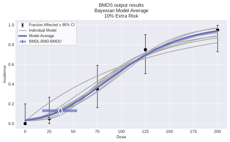
To run ToxicR Bayesian model averaging:

import pybmds
from pybmds.models import dichotomous

# create a dichotomous dataset
dataset = pybmds.DichotomousDataset(
    doses=[0, 25, 75, 125, 200],
    ns=[20, 20, 20, 20, 20],
    incidences=[0, 1, 7, 15, 19],
)

session = pybmds.Session(dataset=dataset)
session.add_default_bayesian_models(
    prior_class=pybmds.PriorClass.bayesian,
    model_average=True,
)
session.execute()

res = session.model_average.results
print(f"BMD = {res.bmd:.2f} [{res.bmdl:.2f}, {res.bmdu:.2f}]")

fig = session.plot(colorize=False)

BMD = 36.65 [17.83, 54.15]

../_images/27f06d3f7f6b8629248aa2c6d9ff37aaddaea81982660d7ef7683acae36a430e.png

Change session settings¶

For a dichotomous Bayesian model average session, the default settings use a BMR of 10% Extra Risk and a 95% confidence interval. To change these settings:

session = pybmds.Session(dataset=dataset)
session.add_default_bayesian_models(
    settings = {
        "bmr": 0.05,
        "bmr_type": pybmds.DichotomousRiskType.AddedRisk,
        "alpha": 0.1
    }
)

This would run the dichotomous models for a BMR of 5% Added Risk at a 90% confidence interval.

Run subset of models¶

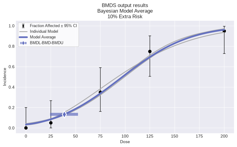
Instead of running all available dichotomous models, you can select a subset of models.

For example, to model average on the Logistic, Probit, and Weibull models:

session = pybmds.Session(dataset=dataset)
session.add_model(pybmds.Models.Weibull, {"priors": pybmds.PriorClass.bayesian})
session.add_model(pybmds.Models.Logistic, {"priors": pybmds.PriorClass.bayesian})
session.add_model(pybmds.Models.Probit, {"priors": pybmds.PriorClass.bayesian})
session.add_model_averaging()

session.execute()

res = session.model_average.results
print(f"BMD = {res.bmd:.2f} [{res.bmdl:.2f}, {res.bmdu:.2f}]")

fig =session.plot(colorize=False)

BMD = 38.54 [24.43, 52.42]

../_images/a648176542b7b062f7d69ef3c8ab6e8999b88958cf72d28c71b06b825187e99c.png

Change parameter settings - ToxicR model averaging¶

You can change the input parameter settings for an analysis.

Running a single Bayesian model with base configuration as an example:

model = dichotomous.Logistic(
    dataset=dataset, settings={"priors": pybmds.PriorClass.bayesian}
)

print(model.settings.tbl())
print(model.priors_tbl())

╒══════════════════════════════╤════════════════╕
│ BMR                          │ 10% Extra Risk │
│ Confidence Level (one sided) │ 0.95           │
│ Modeling approach            │ bayesian       │
│ Degree                       │ 0              │
╘══════════════════════════════╧════════════════╛
╒═════════════╤════════════════╤═════════════════════════════════════════════╕
│ Parameter   │ Distribution   │ Definition                                  │
╞═════════════╪════════════════╪═════════════════════════════════════════════╡
│ a           │ Normal         │ initial=0.0, stdev=2.0, min=-20.0, max=20.0 │
│ b           │ Lognormal      │ initial=0.0, stdev=2.0, min=0.0, max=40.0   │
╘═════════════╧════════════════╧═════════════════════════════════════════════╛

Configuring the model settings or priors:

model = dichotomous.Logistic(
    dataset=dataset,
    settings={
        "priors": pybmds.PriorClass.bayesian,
        "bmr": 0.05
    }
)
model.settings.priors.update('a', stdev=1, min_value=-15, max_value=15)
model.settings.priors.update('b', stdev=3)

print(model.settings.tbl())
print(model.priors_tbl())

╒══════════════════════════════╤═══════════════╕
│ BMR                          │ 5% Extra Risk │
│ Confidence Level (one sided) │ 0.95          │
│ Modeling approach            │ bayesian      │
│ Degree                       │ 0             │
╘══════════════════════════════╧═══════════════╛
╒═════════════╤════════════════╤═════════════════════════════════════════╕
│ Parameter   │ Distribution   │ Definition                              │
╞═════════════╪════════════════╪═════════════════════════════════════════╡
│ a           │ Normal         │ initial=0.0, stdev=1, min=-15, max=15   │
│ b           │ Lognormal      │ initial=0.0, stdev=3, min=0.0, max=40.0 │
╘═════════════╧════════════════╧═════════════════════════════════════════╛

You can also change the parameter prior types from the default listed in the BMDS User Guide. Parameters can be given a Normal, Log-Normal, or Uniform distribution. These can be changed by:

model = dichotomous.Weibull(
    dataset=dataset,
    settings={
        "priors": pybmds.PriorClass.bayesian,
        "bmr": 0.05,
    }
)
model.settings.priors.update(
    'g', type=pybmds.PriorDistribution.Uniform, min_value=0, max_value=1
)
print(model.priors_tbl())

╒═════════════╤════════════════╤════════════════════════════════════════════════╕
│ Parameter   │ Distribution   │ Definition                                     │
╞═════════════╪════════════════╪════════════════════════════════════════════════╡
│ g           │ Uniform        │ initial=0.0, stdev=2.0, min=0, max=1           │
│ a           │ Lognormal      │ initial=0.424264, stdev=0.5, min=0.0, max=40.0 │
│ b           │ Lognormal      │ initial=0.0, stdev=1.5, min=0.0, max=10000.0   │
╘═════════════╧════════════════╧════════════════════════════════════════════════╛

Or:

model.settings.priors.update(
    'g', 
    type=pybmds.PriorDistribution.Lognormal, 
    min_value=0, 
    max_value=1, 
    initial_value=0, 
    stdev=1.5,
)
print(model.priors_tbl())

╒═════════════╤════════════════╤════════════════════════════════════════════════╕
│ Parameter   │ Distribution   │ Definition                                     │
╞═════════════╪════════════════╪════════════════════════════════════════════════╡
│ g           │ Lognormal      │ initial=0, stdev=1.5, min=0, max=1             │
│ a           │ Lognormal      │ initial=0.424264, stdev=0.5, min=0.0, max=40.0 │
│ b           │ Lognormal      │ initial=0.0, stdev=1.5, min=0.0, max=10000.0   │
╘═════════════╧════════════════╧════════════════════════════════════════════════╛