Tumor and Multitumor Data
Table of Contents
Conducting dose-response analysis on dichotomous tumor data differs from analyzing standard dichotomous tumor data in the following ways:
The Multistage cancer model uses different parameter settings for model fit than the standard Multistage model.
A cancer slope factor is calculated.
In some cases, there may be a need to combine multiple tumor datasets and then calculate a single cancer slope factor.
To that end, this guide covers some different approaches that you can use in pybmds for handling tumor data.
Quickstart
To run a single dataset:
import pybmds
from pybmds.models.dichotomous import MultistageCancer
dataset = pybmds.DichotomousDataset(
doses=[0, 25, 75, 125, 200],
ns=[20, 20, 20, 20, 20],
incidences=[0, 1, 7, 15, 19],
name="Tumor dataset A",
dose_units="mg/kg-d",
)
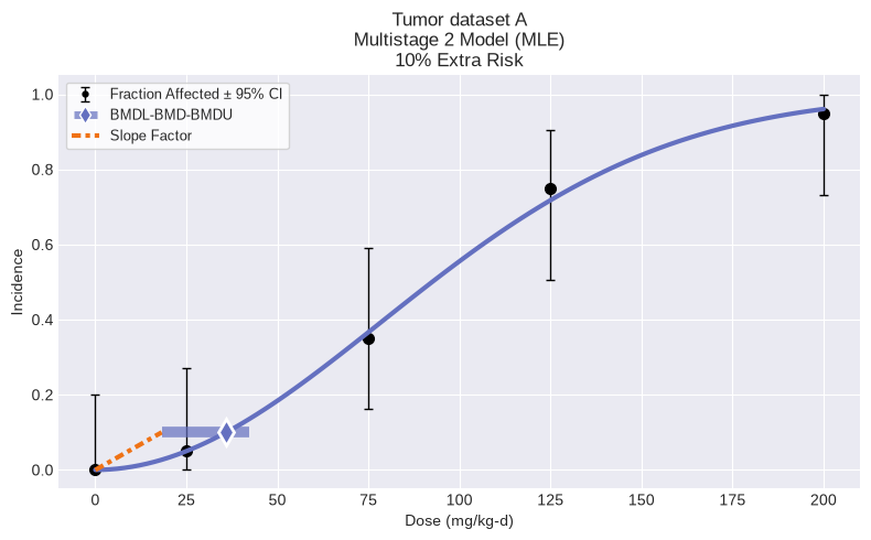
model = MultistageCancer(dataset, settings={"bmr": 0.1})
model.execute(slope_factor=True)
print(f"BMD = {model.results.bmd:f}")
print(f"BMDL = {model.results.bmdl:f}")
print(f"CSF = {model.results.slope_factor:f}")
fig = model.plot()
BMD = 35.929912
BMDL = 18.233585
CSF = 0.005484
To run multiple datasets and calculate a single combined slope factor:
import pybmds

datasets = [
    pybmds.DichotomousDataset(
        doses=[0, 25, 75, 125, 200],
        ns=[20, 20, 20, 20, 20],
        incidences=[0, 1, 7, 15, 19],
        name="Tumor A",
        dose_units="mg/m³",
    ),
    pybmds.DichotomousDataset(
        doses=[0, 25, 75, 125, 200],
        ns=[20, 20, 20, 20, 20],
        incidences=[0, 0, 1, 7, 11],
        name="Tumor B",
        dose_units="mg/m³",
    ),
]

session = pybmds.Multitumor(datasets, settings={"bmr": 0.2}, name="Example")
session.execute()

fig = session.plot()
To view individual model results for selected models for each dataset:
# Print overall results
print("Overall")
print(f"BMD = {session.results.bmd:f}")
print(f"BMDL = {session.results.bmdl:f}")
print(f"CSF = {session.results.slope_factor:f}")
print()

# Print individual model results
selected_model_indexes = session.results.selected_model_indexes
for i, dataset_models in enumerate(session.models):
    selected_index = selected_model_indexes[i]
    selected_model = dataset_models[selected_index]
    print(f"{selected_model.dataset.metadata.name}: {selected_model.name()}")
    print(f"BMD = {selected_model.results.bmd:f}")
    print(f"BMDL = {selected_model.results.bmdl:f}")
    print(f"CSF = {selected_model.results.slope_factor:f}")
    print()
Overall
BMD = 18.835597
BMDL = 15.066557
CSF = 0.013274

Tumor A: Multistage 1
BMD = 24.653310
BMDL = 18.882341
CSF = 0.010592

Tumor B: Multistage 1
BMD = 79.818267
BMDL = 55.735346
CSF = 0.003588
Create a tumor dataset
Create a tumor dataset using the same method as a dichotomous dataset.
As with a dichotomous dataset, provide a list of doses, incidences, and the total number of subjects, one item per dose-group.
You can also add optional attributes, such as name, dose_name, dose_units, response_name, response_units, etc.
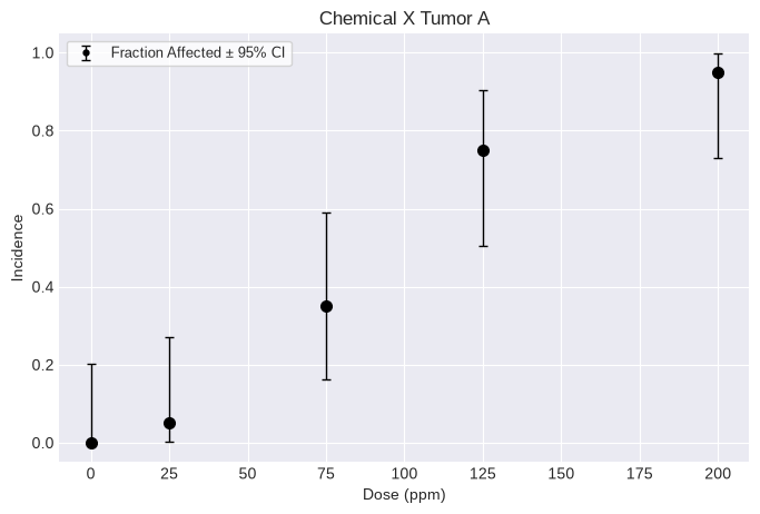
dataset = pybmds.DichotomousDataset(
    name="Chemical X Tumor A",
    dose_units="ppm",
    doses=[0, 25, 75, 125, 200],
    ns=[20, 20, 20, 20, 20],
    incidences=[0, 1, 7, 15, 19],
)

print(dataset.tbl())
fig = dataset.plot()
╒════════╤═════════════╤═════╕
│   Dose │   Incidence │   N │
╞════════╪═════════════╪═════╡
│      0 │           0 │  20 │
│     25 │           1 │  20 │
│     75 │           7 │  20 │
│    125 │          15 │  20 │
│    200 │          19 │  20 │
╘════════╧═════════════╧═════╛
Single dataset fit
With a single tumor dataset defined above, you can run a single Multistage cancer model:
import pybmds
from pybmds.models.dichotomous import MultistageCancer

model = MultistageCancer(dataset, settings={"bmr": 0.10, "degree": 2})
model.execute(slope_factor=True)
fig = model.plot()

After executing, results are stored in a results attribute on the model. You can view individual items in the results by accessing:
print(model.name())
print(f"BMD = {session.results.bmd:f}")
print(f"BMDL = {session.results.bmdl:f}")
print(f"CSF = {session.results.slope_factor:f}")
Multistage 2
BMD = 18.835597
BMDL = 15.066557
CSF = 0.013274
Or generate a text report to view a summary:
print(model.text())
      Multistage 2 Model
══════════════════════════════

Version: pybmds 25.2 (bmdscore 25.2)

Input Summary:
╒══════════════════════════════╤════════════════════════╕
│ BMR                          │ 10% Extra Risk         │
│ Confidence Level (one sided) │ 0.95                   │
│ Modeling approach            │ frequentist_restricted │
│ Degree                       │ 2                      │
╘══════════════════════════════╧════════════════════════╛

Parameter Settings:
╒═════════════╤═══════════╤═══════╤═══════╕
│ Parameter   │   Initial │   Min │   Max │
╞═════════════╪═══════════╪═══════╪═══════╡
│ g           │     -17   │   -18 │    18 │
│ b1          │       0.1 │     0 │ 10000 │
│ b2          │       0.1 │     0 │ 10000 │
╘═════════════╧═══════════╧═══════╧═══════╛

Modeling Summary:
╒════════════════╤══════════════╕
│ BMD            │  35.9299     │
│ BMDL           │  18.2336     │
│ BMDU           │  42.1027     │
│ Slope Factor   │   0.00548438 │
│ AIC            │  68.4561     │
│ Log-Likelihood │ -32.2281     │
│ P-Value        │   0.979879   │
│ Overall d.f.   │   3          │
│ Chi²           │   0.185606   │
╘════════════════╧══════════════╛

Model Parameters:
╒════════════╤═════════════╤════════════╤══════════════╕
│ Variable   │    Estimate │ On Bound   │ Std Error    │
╞════════════╪═════════════╪════════════╪══════════════╡
│ g          │ 1.523e-08   │ yes        │ Not Reported │
│ b1         │ 3.10908e-05 │ no         │ 0.279639     │
│ b2         │ 8.07489e-05 │ no         │ 0.795918     │
╘════════════╧═════════════╧════════════╧══════════════╛
Standard errors estimates are not generated for parameters estimated on corresponding bounds,
although sampling error is present for all parameters, as a rule. Standard error estimates may not
be reliable as a basis for confidence intervals or tests when one or more parameters are on bounds.


Goodness of Fit:
╒════════╤════════╤════════════╤════════════╤════════════╤═══════════════════╕
│   Dose │   Size │   Observed │   Expected │   Est Prob │   Scaled Residual │
╞════════╪════════╪════════════╪════════════╪════════════╪═══════════════════╡
│      0 │     20 │          0 │  3.046e-07 │  1.523e-08 │      -0.000551905 │
│     25 │     20 │          1 │  0.999088  │  0.0499544 │       0.000935604 │
│     75 │     20 │          7 │  7.33062   │  0.366531  │      -0.153425    │
│    125 │     20 │         15 │ 14.3585    │  0.717926  │       0.318744    │
│    200 │     20 │         19 │ 19.2137    │  0.960686  │      -0.245902    │
╘════════╧════════╧════════════╧════════════╧════════════╧═══════════════════╛

Analysis of Deviance:
╒═══════════════╤══════════════════╤════════════╤════════════╤═════════════╤═════════════╕
│ Model         │   Log-Likelihood │   # Params │ Deviance   │ Test d.f.   │ P-Value     │
╞═══════════════╪══════════════════╪════════════╪════════════╪═════════════╪═════════════╡
│ Full model    │         -32.1362 │          5 │ -          │ -           │ -           │
│ Fitted model  │         -32.2281 │          2 │ 0.183639   │ 3           │ 0.980186    │
│ Reduced model │         -68.0292 │          1 │ 71.7859    │ 4           │ 9.54792e-15 │
╘═══════════════╧══════════════════╧════════════╧════════════╧═════════════╧═════════════╛
Change input settings
Model settings can be customized for a run, as with standard dichotomous models.
model = MultistageCancer(
    dataset,
    settings={
        "bmr_type": pybmds.DichotomousRiskType.AddedRisk,
        "bmr": 0.15,
        "degree": 3,
    },
)
print(model.settings.tbl())
╒══════════════════════════════╤════════════════════════╕
│ BMR                          │ 15% Added Risk         │
│ Confidence Level (one sided) │ 0.95                   │
│ Modeling approach            │ frequentist_restricted │
│ Degree                       │ 3                      │
╘══════════════════════════════╧════════════════════════╛
Change parameter settings
Initial parameter settings are different for the MultistageCancer model compared with the dichotomous Multistage:
from pybmds.models.dichotomous import Multistage, MultistageCancer

model = Multistage(dataset)
print("Multistage parameter settings:")
print(model.priors_tbl())

model = MultistageCancer(dataset)
print("Multistage Cancer parameter settings:")
print(model.priors_tbl())
Multistage parameter settings:
╒═════════════╤═══════════╤═══════╤═══════╕
│ Parameter   │   Initial │   Min │   Max │
╞═════════════╪═══════════╪═══════╪═══════╡
│ g           │         0 │   -18 │    18 │
│ b1          │         0 │     0 │ 10000 │
│ b2          │         0 │     0 │ 10000 │
╘═════════════╧═══════════╧═══════╧═══════╛
Multistage Cancer parameter settings:
╒═════════════╤═══════════╤═══════╤═══════╕
│ Parameter   │   Initial │   Min │   Max │
╞═════════════╪═══════════╪═══════╪═══════╡
│ g           │     -17   │   -18 │    18 │
│ b1          │       0.1 │     0 │ 10000 │
│ b2          │       0.1 │     0 │ 10000 │
╘═════════════╧═══════════╧═══════╧═══════╛
For Multistage models, the b2 parameter setting is reused for all beta parameters greater than or equal to b2.
These can be updated:
model.settings.priors.update("g", initial_value=0, min_value=-10, max_value=10)
model.settings.priors.update("b1", initial_value=10, min_value=0, max_value=100)
model.settings.priors.update("b2", initial_value=20, min_value=0, max_value=1000)

print(model.priors_tbl())
╒═════════════╤═══════════╤═══════╤═══════╕
│ Parameter   │   Initial │   Min │   Max │
╞═════════════╪═══════════╪═══════╪═══════╡
│ g           │         0 │   -10 │    10 │
│ b1          │        10 │     0 │   100 │
│ b2          │        20 │     0 │  1000 │
╘═════════════╧═══════════╧═══════╧═══════╛
Fit multiple models
The previous example runs a single Multitumor model to a single dataset. However, you may want, for example, to run multiple multitumor models of varying degrees to a single dataset.
Multiple dataset fit
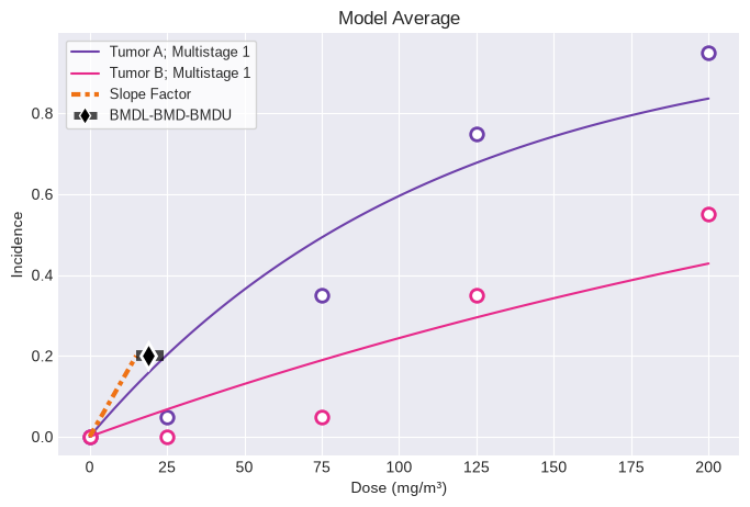
To fit multiple models and one or more datasets, use an instance of the Multitumor class:
import pybmds

datasets = [
    pybmds.DichotomousDataset(
        doses=[0, 25, 75, 125, 200],
        ns=[20, 20, 20, 20, 20],
        incidences=[0, 1, 7, 15, 19],
        name="Tumor A",
        dose_units="mg/m³",
    ),
    pybmds.DichotomousDataset(
        doses=[0, 25, 75, 125, 200],
        ns=[20, 20, 20, 20, 20],
        incidences=[0, 0, 1, 7, 11],
        name="Tumor B",
        dose_units="mg/m³",
    ),
]

session = pybmds.Multitumor(datasets)
session.execute()

print(session.results.tbl())
fig = session.plot()
╒══════════════════════════════════╤════════════╕
│ BMD                              │   8.8935   │
│ BMDL                             │   7.1139   │
│ BMDU                             │  11.2427   │
│ Slope Factor                     │   0.014057 │
│ Combined Log-likelihood          │ -70.8752   │
│ Combined Log-likelihood Constant │ -53.1841   │
╘══════════════════════════════════╧════════════╛
You can generate Excel and Word exports:
# save excel report
df = session.to_df()
df.to_excel("output/report.xlsx")

# save to a word report
report = session.to_docx()
report.save("output/report.docx")
Change model settings
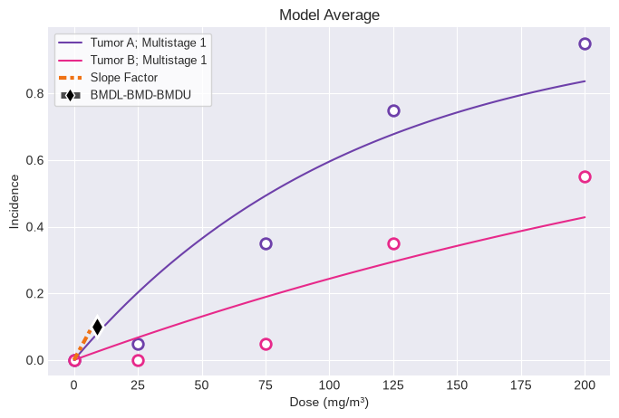
Settings for all datasets and models should be configured globally and are applied to all models:
session = pybmds.Multitumor(datasets, settings={
    "bmr_type": pybmds.DichotomousRiskType.AddedRisk,
    "bmr": 0.15,
})
Change model degree
By default, multiple models are executed for each dataset, where the degree is varied from 1 to the number of doses minus 1 (and a maximum of 8).
For this example, we first create three datasets:
datasets = [
    pybmds.DichotomousDataset(
        doses=[0, 2, 3, 4, 5, 6, 7, 8, 9],
        ns=[20, 20, 20, 20, 20, 20, 20, 20, 20],
        incidences=[0, 1, 4, 8, 11, 12, 13, 14, 15],
        name="Tumor A (9 groups)",
        dose_units="mg/m³",
    ),
    pybmds.DichotomousDataset(
        doses=[0, 2, 3, 4, 5, 6, 7, 8, 9],
        ns=[20, 20, 20, 20, 20, 20, 20, 20, 20],
        incidences=[0, 1, 7, 15, 19, 19, 19, 19, 19],
        name="Tumor B (9 groups)",
        dose_units="mg/m³",
    ),
    pybmds.DichotomousDataset(
        doses=[0, 2, 3, 4, 5],
        ns=[20, 20, 20, 20, 20],
        incidences=[0, 0, 1, 7, 11],
        name="Tumor C (5 groups)",
        dose_units="mg/m³",
    ),
]
Next, we specify which model degrees to run for each dataset using degrees. Setting a value of 0 runs all degrees available up to a maximum of 8; specifying a specific degree will only run the specified degree.
degrees = [0, 3, 2]
session = pybmds.Multitumor(datasets, degrees=degrees)
session.execute()
fig = session.plot()
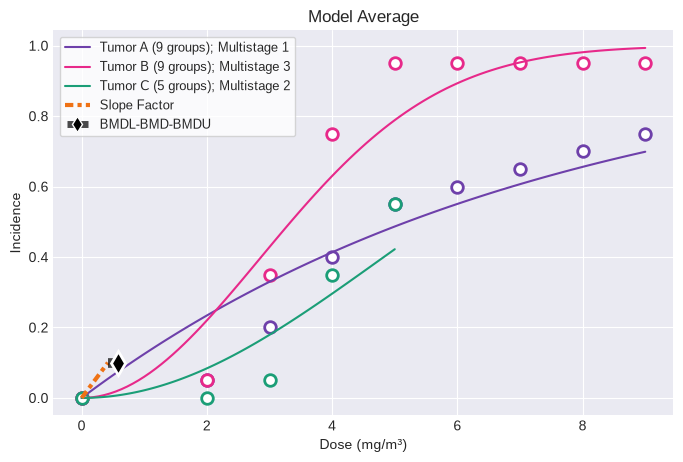
The analysis executed the following models for each dataset:
for dataset_models in session.models:
    print(f"{dataset_models[0].dataset.metadata.name}")
    for model in dataset_models:
        print("\t" + model.name())
Tumor A (9 groups)
	Multistage 1
	Multistage 2
	Multistage 3
	Multistage 4
	Multistage 5
	Multistage 6
	Multistage 7
	Multistage 8
Tumor B (9 groups)
	Multistage 3
Tumor C (5 groups)
	Multistage 2
Note that the Multistage and MultistageCancer models both use the standard model selection workflow for dichotomous data (see BMDS User Guide), whereas the Multitumor model uses a modifed workflow specific to use of the multistage model specifically for cancer endpoints. If users would like to apply the modified Multistage model selection workflow on individual tumors, they can simply run the Multitumor model on single tumor datasets.
For illustration, consider the dataset below, modeled with the Multistage Cancer model:
from pybmds.models.dichotomous import MultistageCancer

esophogeal_tumors_female = pybmds.DichotomousDataset(
        doses=[0, 0.002, 0.004, 0.009, 0.018, 0.036, 0.072, 0.107, 0.143],
        ns=[240, 60, 60, 60, 60, 60, 60, 60, 60],
        incidences=[0, 0, 0, 0, 0, 0, 2, 8, 16],
        name="Esophogeal tumors - females",
        dose_units="mg/kg-d",
)

model = MultistageCancer(dataset, settings={"bmr": 0.1})
model.execute(slope_factor=True)

print(f"BMD = {model.results.bmd:f}")
print(f"BMDL = {model.results.bmdl:f}")
print(f"CSF = {model.results.slope_factor:f}")

fig = model.plot()
print(model.text())
BMD = 35.929912
BMDL = 18.233585
CSF = 0.005484
      Multistage 2 Model
══════════════════════════════

Version: pybmds 25.2 (bmdscore 25.2)

Input Summary:
╒══════════════════════════════╤════════════════════════╕
│ BMR                          │ 10% Extra Risk         │
│ Confidence Level (one sided) │ 0.95                   │
│ Modeling approach            │ frequentist_restricted │
│ Degree                       │ 2                      │
╘══════════════════════════════╧════════════════════════╛

Parameter Settings:
╒═════════════╤═══════════╤═══════╤═══════╕
│ Parameter   │   Initial │   Min │   Max │
╞═════════════╪═══════════╪═══════╪═══════╡
│ g           │     -17   │   -18 │    18 │
│ b1          │       0.1 │     0 │ 10000 │
│ b2          │       0.1 │     0 │ 10000 │
╘═════════════╧═══════════╧═══════╧═══════╛

Modeling Summary:
╒════════════════╤══════════════╕
│ BMD            │  35.9299     │
│ BMDL           │  18.2336     │
│ BMDU           │  42.1027     │
│ Slope Factor   │   0.00548438 │
│ AIC            │  68.4561     │
│ Log-Likelihood │ -32.2281     │
│ P-Value        │   0.979879   │
│ Overall d.f.   │   3          │
│ Chi²           │   0.185606   │
╘════════════════╧══════════════╛

Model Parameters:
╒════════════╤═════════════╤════════════╤══════════════╕
│ Variable   │    Estimate │ On Bound   │ Std Error    │
╞════════════╪═════════════╪════════════╪══════════════╡
│ g          │ 1.523e-08   │ yes        │ Not Reported │
│ b1         │ 3.10908e-05 │ no         │ 0.279639     │
│ b2         │ 8.07489e-05 │ no         │ 0.795918     │
╘════════════╧═════════════╧════════════╧══════════════╛
Standard errors estimates are not generated for parameters estimated on corresponding bounds,
although sampling error is present for all parameters, as a rule. Standard error estimates may not
be reliable as a basis for confidence intervals or tests when one or more parameters are on bounds.


Goodness of Fit:
╒════════╤════════╤════════════╤════════════╤════════════╤═══════════════════╕
│   Dose │   Size │   Observed │   Expected │   Est Prob │   Scaled Residual │
╞════════╪════════╪════════════╪════════════╪════════════╪═══════════════════╡
│      0 │     20 │          0 │  3.046e-07 │  1.523e-08 │      -0.000551905 │
│     25 │     20 │          1 │  0.999088  │  0.0499544 │       0.000935604 │
│     75 │     20 │          7 │  7.33062   │  0.366531  │      -0.153425    │
│    125 │     20 │         15 │ 14.3585    │  0.717926  │       0.318744    │
│    200 │     20 │         19 │ 19.2137    │  0.960686  │      -0.245902    │
╘════════╧════════╧════════════╧════════════╧════════════╧═══════════════════╛

Analysis of Deviance:
╒═══════════════╤══════════════════╤════════════╤════════════╤═════════════╤═════════════╕
│ Model         │   Log-Likelihood │   # Params │ Deviance   │ Test d.f.   │ P-Value     │
╞═══════════════╪══════════════════╪════════════╪════════════╪═════════════╪═════════════╡
│ Full model    │         -32.1362 │          5 │ -          │ -           │ -           │
│ Fitted model  │         -32.2281 │          2 │ 0.183639   │ 3           │ 0.980186    │
│ Reduced model │         -68.0292 │          1 │ 71.7859    │ 4           │ 9.54792e-15 │
╘═══════════════╧══════════════════╧════════════╧════════════╧═════════════╧═════════════╛
In this case, the 2nd degree Multistage model has been selected based on the standard dichotomous model selection workflow.
If this same tumor dataset was modeled along with another tumor dataset with the Multitumor model, the results would be:
hepatocellular_tumors_female = pybmds.DichotomousDataset(
    doses=[0, 0.002, 0.004, 0.009, 0.018, 0.036, 0.072, 0.107],
    ns=[240, 60, 60, 60, 60, 60, 60, 60],
    incidences=[13, 4, 6, 3, 6, 11, 35, 48],
    name="Hepatocellular tumors - females",
    dose_units="mg/kg-d",
)

datasets = [
    hepatocellular_tumors_female,
    esophogeal_tumors_female
]

session = pybmds.Multitumor(datasets)
session.execute()

print(session.results.tbl())
fig = session.plot()
╒══════════════════════════════════╤═══════════════╕
│ BMD                              │     0.0234891 │
│ BMDL                             │     0.021427  │
│ BMDU                             │     0.0234891 │
│ Slope Factor                     │     4.667     │
│ Combined Log-likelihood          │  -292.531     │
│ Combined Log-likelihood Constant │ -9999         │
╘══════════════════════════════════╧═══════════════╛
nlopt failed: bounds 0 fail -1.80631 <= -1.80631 <= -1.94491
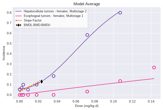
Observe that when the esophogeal tumors are modeled with the Multitumor model, the 1st degree Multistage model is selected using the modified Multistage model selection workflow.
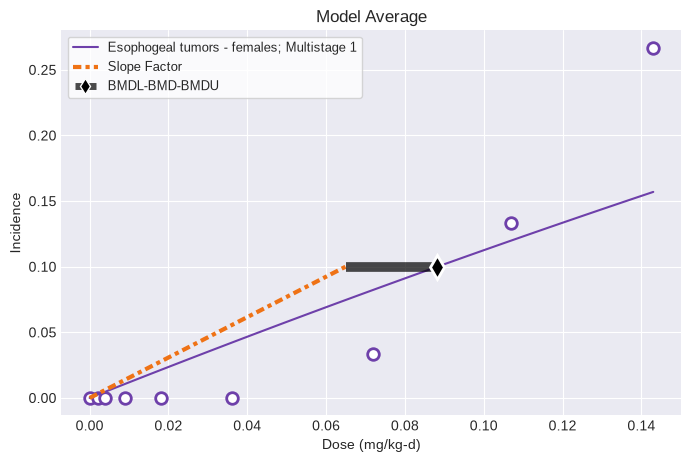
Users can apply the modified workflow to single tumor datasets by simply running the Multitumor model on indiviudal datasets:
datasets = [esophogeal_tumors_female]
session = pybmds.Multitumor(datasets)
session.execute()

print(session.results.tbl())
fig = session.plot()
nlopt failed: bounds 0 fail -0.482868 <= -0.482868 <= -1.94491
╒══════════════════════════════════╤═══════════════╕
│ BMD                              │     0.0882326 │
│ BMDL                             │     0.0649418 │
│ BMDU                             │     0.0882326 │
│ Slope Factor                     │     1.53984   │
│ Combined Log-likelihood          │   -75.673     │
│ Combined Log-likelihood Constant │ -9999         │
╘══════════════════════════════════╧═══════════════╛
PolyK Adjustment for Early Mortality
Often, in cancer bioassays, exposure to the carcinogen of interest will result in differential survival across exposure groups, with animals in higher exposure groups dying for frequently and at earlier time points. If this is not taken into account, the unadjusted data will underestimate the true proportion of animals developing the tumor of incidence and risks will be also be underestimated. See BMDS User Guide for full details on the PolyK adjustment methods.
Consider a tumor dataset saved as a CSV with dose, day of death, and tumor status (i.e., 1 = has tumor and 0 = no tumor):
import pandas as pd

df = pd.read_csv('data/example-polyk.csv')
df.head()
| dose | day | has_tumor | |
|---|---|---|---|
| 0 | 0.0 | 452 | 0 |
| 1 | 0.0 | 535 | 0 |
| 2 | 0.0 | 553 | 0 |
| 3 | 0.0 | 570 | 0 |
| 4 | 0.0 | 596 | 0 |
The PolyK adjustment can be run by calling the PolyKAdjustment class. Note that the columns in your csv corresponding to doses, days, and has_tumor variables must be defined. The polynomial degree (k) can be set by the user, but the method defaults to a value of 3. The maximum number of days on test in the bioassay (max_days) can also be manually defined by the user, but this variable will automatically be set to the highest value in the days column otherwise.
from pybmds.datasets.transforms.polyk import PolyKAdjustment

# Define which columns in the dataframe correspond to dose, time (day), and response (has_tumor)
doses = df["dose"].tolist()
days = df["day"].tolist()
has_tumor = df["has_tumor"].tolist()

# Create an instance of PolyKAdjustment
poly_k = PolyKAdjustment(
    doses=doses,
    day=days,
    has_tumor=has_tumor,
    k=3,                # Optional, default is 3
    max_day=None,       # Optional, will use max day from data if None
    dose_units="",
    dose_name="Dose",
    time_units="days"
)

# Print summary table to see adjusted N and proportions
print(poly_k.summary)

# Plot summary figure
fig1 = poly_k.summary_figure()
fig2 = poly_k.tumor_incidence_figure()
   dose     n      adj_n  incidence  proportion  adj_proportion
0   0.0  50.0  42.421583        6.0        0.12        0.141437
1  12.8  50.0  42.303325       12.0        0.24        0.283666
2  32.0  50.0  40.347370       23.0        0.46        0.570050
3  80.0  50.0  42.144682       28.0        0.56        0.664378
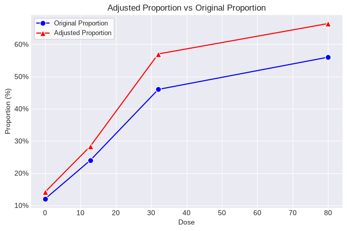
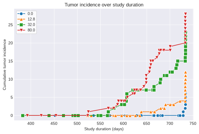
The adjusted Ns and original incidence values can now be used in a MultistageCancer or Multitumor analysis and the resulting BMD, BMDL, and cancer slope factor will reflect the increased proportion of tumor-bearing animals due to differential survival across dose groups.