Nested Dichotomous Data
Table of Contents
Quickstart
To run a nested dichotomous dataset:
import pybmds

dataset = pybmds.NestedDichotomousDataset(
    name="Nested Dataset",
    dose_units="ppm",
    doses= [
        0, 0, 0, 0, 0, 0, 0, 0, 0, 0,
        25, 25, 25, 25, 25, 25, 25, 25, 25, 25,
        50, 50, 50, 50, 50, 50, 50, 50, 50, 50,
        100, 100, 100, 100, 100, 100, 100, 100, 100
    ],
    litter_ns = [
        16, 9, 15, 14, 13, 9, 10, 14, 10, 11,
        14, 9, 14, 9, 13, 12, 10, 10, 11, 14,
        11, 11, 14, 11, 10, 11, 10, 15, 7, 14,
        11, 14, 12, 13, 12, 14, 11, 8, 10
    ],
    incidences = [
        1, 1, 2, 3, 3, 0, 2, 2, 1, 2,
        4, 5, 6, 2, 6, 3, 1, 2, 4, 3,
        4, 5, 5, 4, 5, 4, 5, 6, 2, 4,
        6, 6, 8, 7, 8, 6, 6, 5, 4
    ],
    litter_covariates = [
        16, 9, 15, 14, 13, 9, 10, 14, 10, 11,
        14, 9, 14, 9, 13, 12, 10, 10, 11, 14,
        11, 11, 14, 11, 10, 11, 10, 15, 7, 14,
        11, 14, 12, 13, 12, 14, 11, 8, 10
    ]
)

# create a BMD session
session = pybmds.Session(dataset=dataset)

# add all default models
session.add_default_models()

# execute the session
session.execute_and_recommend()

# recommend a best-fitting model
session.recommend()

if session.recommended_model is not None:
    fig = session.recommended_model.plot()
    print(session.recommended_model.text())

# save excel report
df = session.to_df()
df.to_excel("output/nd-report.xlsx")

# save to a word report
report = session.to_docx()
report.save("output/nd-report.docx")
Nested Logistic (lsc+ilc+) Model
══════════════════════════════

Version: pybmds 25.2 (bmdscore 25.2)

Input Summary:
╒══════════════════════════════╤═══════════════════════╕
│ BMR                          │ 5% Extra Risk         │
│ Confidence Level (one sided) │ 0.95                  │
│ Litter Specific Covariate    │ Overall Mean (11.692) │
│ Intralitter Correlation      │ Estimate              │
│ Estimate Background          │ True                  │
│ Bootstrap Runs               │ 3                     │
│ Bootstrap Iterations         │ 1000                  │
│ Bootstrap Seed               │ 878                   │
╘══════════════════════════════╧═══════════════════════╛

Parameter Settings:
╒═════════════╤═══════════╤═══════╤════════╕
│ Parameter   │   Initial │   Min │    Max │
╞═════════════╪═══════════╪═══════╪════════╡
│ a           │         0 │     0 │  1     │
│ b           │         0 │   -18 │ 18     │
│ theta1      │         0 │     0 │  1     │
│ theta2      │         0 │   -18 │ 18     │
│ rho         │         1 │     1 │ 18     │
│ phi1        │         0 │     0 │  1e+06 │
│ phi2        │         0 │     0 │  1e+06 │
│ phi3        │         0 │     0 │  1e+06 │
│ phi4        │         0 │     0 │  1e+06 │
╘═════════════╧═══════════╧═══════╧════════╛

Modeling Summary:
╒════════════════╤═════════════╕
│ BMD            │    6.13674  │
│ BMDL           │    4.56796  │
│ BMDU           │    9.20512  │
│ AIC            │  546.957    │
│ P-Value        │    0.998667 │
│ d.f.           │   35        │
│ Chi²           │   19.6089   │
│ Log-Likelihood │ -269.479    │
╘════════════════╧═════════════╛

Model Parameters:
╒════════════╤═════════════╤════════════╤══════════════╕
│ Variable   │    Estimate │ On Bound   │ Std Error    │
╞════════════╪═════════════╪════════════╪══════════════╡
│ a          │  0.0847489  │ no         │ 0.0822572    │
│ b          │ -4.11365    │ no         │ 1.11128      │
│ theta1     │  0.00476225 │ no         │ 0.0588407    │
│ theta2     │ -0.0551719  │ no         │ 0.0924933    │
│ rho        │  1          │ yes        │ Not Reported │
│ phi1       │  0          │ yes        │ Not Reported │
│ phi2       │  0          │ yes        │ Not Reported │
│ phi3       │  0          │ yes        │ Not Reported │
│ phi4       │  0          │ yes        │ Not Reported │
╘════════════╧═════════════╧════════════╧══════════════╛
Standard errors estimates are not generated for parameters estimated on corresponding bounds,
although sampling error is present for all parameters, as a rule. Standard error estimates may not
be reliable as a basis for confidence intervals or tests when one or more parameters are on bounds.


Bootstrap Runs:
╒══════════╤═══════════╤═════════╤═════════╤═════════╤═════════╕
│ Run      │   P-Value │    50th │    90th │    95th │    99th │
╞══════════╪═══════════╪═════════╪═════════╪═════════╪═════════╡
│ 1        │  0.998    │ 38.5389 │ 51.0938 │ 56.0989 │ 62.4221 │
│ 2        │  0.998    │ 37.9941 │ 50.2309 │ 54.2097 │ 61.65   │
│ 3        │  1        │ 37.9496 │ 49.3409 │ 53.7736 │ 60.9342 │
│ Combined │  0.998667 │ 38.1095 │ 50.0054 │ 54.772  │ 61.415  │
╘══════════╧═══════════╧═════════╧═════════╧═════════╧═════════╛

Scaled Residuals (for dose group nearest the BMD):
╒══════════════════════════════╤══════════╕
│ Minimum scaled residual      │ 0.430833 │
│ Minimum ABS(scaled residual) │ 0.430833 │
│ Average scaled residual      │ 0.430833 │
│ Average ABS(scaled residual) │ 0.430833 │
│ Maximum scaled residual      │ 0.430833 │
│ Maximum ABS(scaled residual) │ 0.430833 │
╘══════════════════════════════╧══════════╛

Litter Data:
╒════════╤═══════╤══════════════╤════════════╤════════════╤════════════╤═══════════════════╕
│   Dose │   LSC │   Est. Prob. │   Litter N │   Expected │   Observed │   Scaled Residual │
╞════════╪═══════╪══════════════╪════════════╪════════════╪════════════╪═══════════════════╡
│      0 │     9 │     0.127609 │          9 │    1.14848 │          0 │       -1.14738    │
│      0 │     9 │     0.127609 │          9 │    1.14848 │          1 │       -0.14834    │
│      0 │    10 │     0.132371 │         10 │    1.32371 │          1 │       -0.302063   │
│      0 │    10 │     0.132371 │         10 │    1.32371 │          2 │        0.631053   │
│      0 │    11 │     0.137134 │         11 │    1.50847 │          2 │        0.430833   │
│      0 │    13 │     0.146658 │         13 │    1.90656 │          3 │        0.857255   │
│      0 │    14 │     0.15142  │         14 │    2.11989 │          2 │       -0.0893856  │
│      0 │    14 │     0.15142  │         14 │    2.11989 │          3 │        0.6562     │
│      0 │    15 │     0.156183 │         15 │    2.34274 │          2 │       -0.24377    │
│      0 │    16 │     0.160945 │         16 │    2.57512 │          1 │       -1.07157    │
│     25 │     9 │     0.301387 │          9 │    2.71249 │          2 │       -0.517576   │
│     25 │     9 │     0.301387 │          9 │    2.71249 │          5 │        1.66174    │
│     25 │    10 │     0.297691 │         10 │    2.97691 │          1 │       -1.36723    │
│     25 │    10 │     0.297691 │         10 │    2.97691 │          2 │       -0.675631   │
│     25 │    11 │     0.294329 │         11 │    3.23762 │          4 │        0.504382   │
│     25 │    12 │     0.291293 │         12 │    3.49552 │          3 │       -0.314826   │
│     25 │    13 │     0.288578 │         13 │    3.75151 │          6 │        1.37633    │
│     25 │    14 │     0.286176 │         14 │    4.00646 │          3 │       -0.595141   │
│     25 │    14 │     0.286176 │         14 │    4.00646 │          4 │       -0.00381924 │
│     25 │    14 │     0.286176 │         14 │    4.00646 │          6 │        1.17882    │
│     50 │     7 │     0.433046 │          7 │    3.03132 │          2 │       -0.786693   │
│     50 │    10 │     0.410094 │         10 │    4.10094 │          5 │        0.578039   │
│     50 │    10 │     0.410094 │         10 │    4.10094 │          5 │        0.578039   │
│     50 │    11 │     0.403075 │         11 │    4.43383 │          4 │       -0.266666   │
│     50 │    11 │     0.403075 │         11 │    4.43383 │          4 │       -0.266666   │
│     50 │    11 │     0.403075 │         11 │    4.43383 │          4 │       -0.266666   │
│     50 │    11 │     0.403075 │         11 │    4.43383 │          5 │        0.348016   │
│     50 │    14 │     0.383997 │         14 │    5.37596 │          4 │       -0.756114   │
│     50 │    14 │     0.383997 │         14 │    5.37596 │          5 │       -0.206598   │
│     50 │    15 │     0.378308 │         15 │    5.67462 │          6 │        0.173233   │
│    100 │     8 │     0.572418 │          8 │    4.57935 │          5 │        0.300618   │
│    100 │    10 │     0.553133 │         10 │    5.53133 │          4 │       -0.974012   │
│    100 │    11 │     0.543708 │         11 │    5.98079 │          6 │        0.0116311  │
│    100 │    11 │     0.543708 │         11 │    5.98079 │          6 │        0.0116311  │
│    100 │    12 │     0.534451 │         12 │    6.41342 │          8 │        0.918197   │
│    100 │    12 │     0.534451 │         12 │    6.41342 │          8 │        0.918197   │
│    100 │    13 │     0.52538  │         13 │    6.82994 │          7 │        0.0944518  │
│    100 │    14 │     0.516511 │         14 │    7.23115 │          6 │       -0.658439   │
│    100 │    14 │     0.516511 │         14 │    7.23115 │          6 │       -0.658439   │
╘════════╧═══════╧══════════════╧════════════╧════════════╧════════════╧═══════════════════╛
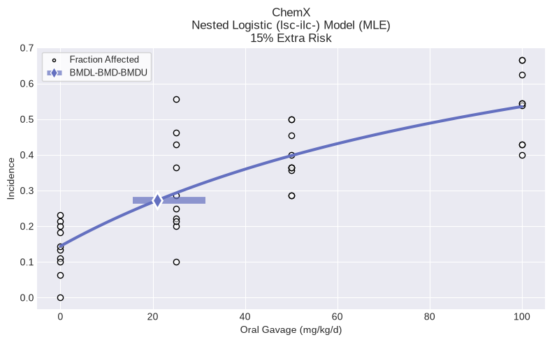
Nested dichotomous dataset
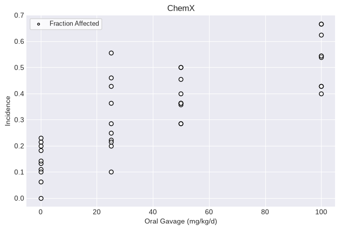
Creating a nested dichotomous dataset requires a list of doses, litter Ns, incidence, and litter covariates. All lists must have the same number of items, with the total items equal to the total number of litters.
You can also add optional attributes, such as name, dose_name, dose_units, response_name, response_units, etc.
dataset = pybmds.NestedDichotomousDataset(
    name="ChemX",
    dose_name="Oral Gavage",
    dose_units="mg/kg/d",
    doses= [
        0, 0, 0, 0, 0, 0, 0, 0, 0, 0,
        25, 25, 25, 25, 25, 25, 25, 25, 25, 25,
        50, 50, 50, 50, 50, 50, 50, 50, 50, 50,
        100, 100, 100, 100, 100, 100, 100, 100, 100
    ],
    litter_ns = [
        16, 9, 15, 14, 13, 9, 10, 14, 10, 11,
        14, 9, 14, 9, 13, 12, 10, 10, 11, 14,
        11, 11, 14, 11, 10, 11, 10, 15, 7, 14,
        11, 14, 12, 13, 12, 14, 11, 8, 10
    ],
    incidences = [
        1, 1, 2, 3, 3, 0, 2, 2, 1, 2,
        4, 5, 6, 2, 6, 3, 1, 2, 4, 3,
        4, 5, 5, 4, 5, 4, 5, 6, 2, 4,
        6, 6, 8, 7, 8, 6, 6, 5, 4
    ],
    litter_covariates = [
        16, 9, 15, 14, 13, 9, 10, 14, 10, 11,
        14, 9, 14, 9, 13, 12, 10, 10, 11, 14,
        11, 11, 14, 11, 10, 11, 10, 15, 7, 14,
        11, 14, 12, 13, 12, 14, 11, 8, 10
    ]
)

fig = dataset.plot()
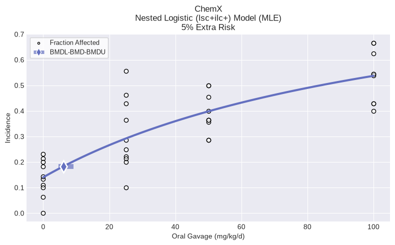
Single model fit
If you want to fit only one model to your dataset, you can fit the specific model to the dataset and print the results, such as the BMD, BMDL, BMDU, p-value, AIC, etc.
For example, to execute the Nested Logistic model:
from pybmds.models import nested_dichotomous

model = nested_dichotomous.NestedLogistic(dataset)
model.execute()
fig = model.plot()
An output report can be generated after execution:
print(model.text())
Nested Logistic (lsc+ilc+) Model
══════════════════════════════

Version: pybmds 25.2 (bmdscore 25.2)

Input Summary:
╒══════════════════════════════╤═══════════════════════╕
│ BMR                          │ 5% Extra Risk         │
│ Confidence Level (one sided) │ 0.95                  │
│ Litter Specific Covariate    │ Overall Mean (11.692) │
│ Intralitter Correlation      │ Estimate              │
│ Estimate Background          │ True                  │
│ Bootstrap Runs               │ 3                     │
│ Bootstrap Iterations         │ 1000                  │
│ Bootstrap Seed               │ 223                   │
╘══════════════════════════════╧═══════════════════════╛

Parameter Settings:
╒═════════════╤═══════════╤═══════╤════════╕
│ Parameter   │   Initial │   Min │    Max │
╞═════════════╪═══════════╪═══════╪════════╡
│ a           │         0 │     0 │  1     │
│ b           │         0 │   -18 │ 18     │
│ theta1      │         0 │     0 │  1     │
│ theta2      │         0 │   -18 │ 18     │
│ rho         │         1 │     1 │ 18     │
│ phi1        │         0 │     0 │  1e+06 │
│ phi2        │         0 │     0 │  1e+06 │
│ phi3        │         0 │     0 │  1e+06 │
│ phi4        │         0 │     0 │  1e+06 │
╘═════════════╧═══════════╧═══════╧════════╛

Modeling Summary:
╒════════════════╤════════════╕
│ BMD            │    6.13674 │
│ BMDL           │    4.56796 │
│ BMDU           │    9.20512 │
│ AIC            │  546.957   │
│ P-Value        │    0.997   │
│ d.f.           │   35       │
│ Chi²           │   19.6089  │
│ Log-Likelihood │ -269.479   │
╘════════════════╧════════════╛

Model Parameters:
╒════════════╤═════════════╤════════════╤══════════════╕
│ Variable   │    Estimate │ On Bound   │ Std Error    │
╞════════════╪═════════════╪════════════╪══════════════╡
│ a          │  0.0847489  │ no         │ 0.0822572    │
│ b          │ -4.11365    │ no         │ 1.11128      │
│ theta1     │  0.00476225 │ no         │ 0.0588407    │
│ theta2     │ -0.0551719  │ no         │ 0.0924933    │
│ rho        │  1          │ yes        │ Not Reported │
│ phi1       │  0          │ yes        │ Not Reported │
│ phi2       │  0          │ yes        │ Not Reported │
│ phi3       │  0          │ yes        │ Not Reported │
│ phi4       │  0          │ yes        │ Not Reported │
╘════════════╧═════════════╧════════════╧══════════════╛
Standard errors estimates are not generated for parameters estimated on corresponding bounds,
although sampling error is present for all parameters, as a rule. Standard error estimates may not
be reliable as a basis for confidence intervals or tests when one or more parameters are on bounds.


Bootstrap Runs:
╒══════════╤═══════════╤═════════╤═════════╤═════════╤═════════╕
│ Run      │   P-Value │    50th │    90th │    95th │    99th │
╞══════════╪═══════════╪═════════╪═════════╪═════════╪═════════╡
│ 1        │     0.995 │ 38.3219 │ 50.4015 │ 53.3503 │ 61.6949 │
│ 2        │     0.999 │ 38.3229 │ 50.379  │ 54.6561 │ 63.3384 │
│ 3        │     0.997 │ 38.5618 │ 50.1832 │ 53.5221 │ 65.3434 │
│ Combined │     0.997 │ 38.371  │ 50.227  │ 53.6788 │ 63.2487 │
╘══════════╧═══════════╧═════════╧═════════╧═════════╧═════════╛

Scaled Residuals (for dose group nearest the BMD):
╒══════════════════════════════╤══════════╕
│ Minimum scaled residual      │ 0.430833 │
│ Minimum ABS(scaled residual) │ 0.430833 │
│ Average scaled residual      │ 0.430833 │
│ Average ABS(scaled residual) │ 0.430833 │
│ Maximum scaled residual      │ 0.430833 │
│ Maximum ABS(scaled residual) │ 0.430833 │
╘══════════════════════════════╧══════════╛

Litter Data:
╒════════╤═══════╤══════════════╤════════════╤════════════╤════════════╤═══════════════════╕
│   Dose │   LSC │   Est. Prob. │   Litter N │   Expected │   Observed │   Scaled Residual │
╞════════╪═══════╪══════════════╪════════════╪════════════╪════════════╪═══════════════════╡
│      0 │     9 │     0.127609 │          9 │    1.14848 │          0 │       -1.14738    │
│      0 │     9 │     0.127609 │          9 │    1.14848 │          1 │       -0.14834    │
│      0 │    10 │     0.132371 │         10 │    1.32371 │          1 │       -0.302063   │
│      0 │    10 │     0.132371 │         10 │    1.32371 │          2 │        0.631053   │
│      0 │    11 │     0.137134 │         11 │    1.50847 │          2 │        0.430833   │
│      0 │    13 │     0.146658 │         13 │    1.90656 │          3 │        0.857255   │
│      0 │    14 │     0.15142  │         14 │    2.11989 │          2 │       -0.0893856  │
│      0 │    14 │     0.15142  │         14 │    2.11989 │          3 │        0.6562     │
│      0 │    15 │     0.156183 │         15 │    2.34274 │          2 │       -0.24377    │
│      0 │    16 │     0.160945 │         16 │    2.57512 │          1 │       -1.07157    │
│     25 │     9 │     0.301387 │          9 │    2.71249 │          2 │       -0.517576   │
│     25 │     9 │     0.301387 │          9 │    2.71249 │          5 │        1.66174    │
│     25 │    10 │     0.297691 │         10 │    2.97691 │          1 │       -1.36723    │
│     25 │    10 │     0.297691 │         10 │    2.97691 │          2 │       -0.675631   │
│     25 │    11 │     0.294329 │         11 │    3.23762 │          4 │        0.504382   │
│     25 │    12 │     0.291293 │         12 │    3.49552 │          3 │       -0.314826   │
│     25 │    13 │     0.288578 │         13 │    3.75151 │          6 │        1.37633    │
│     25 │    14 │     0.286176 │         14 │    4.00646 │          3 │       -0.595141   │
│     25 │    14 │     0.286176 │         14 │    4.00646 │          4 │       -0.00381924 │
│     25 │    14 │     0.286176 │         14 │    4.00646 │          6 │        1.17882    │
│     50 │     7 │     0.433046 │          7 │    3.03132 │          2 │       -0.786693   │
│     50 │    10 │     0.410094 │         10 │    4.10094 │          5 │        0.578039   │
│     50 │    10 │     0.410094 │         10 │    4.10094 │          5 │        0.578039   │
│     50 │    11 │     0.403075 │         11 │    4.43383 │          4 │       -0.266666   │
│     50 │    11 │     0.403075 │         11 │    4.43383 │          4 │       -0.266666   │
│     50 │    11 │     0.403075 │         11 │    4.43383 │          4 │       -0.266666   │
│     50 │    11 │     0.403075 │         11 │    4.43383 │          5 │        0.348016   │
│     50 │    14 │     0.383997 │         14 │    5.37596 │          4 │       -0.756114   │
│     50 │    14 │     0.383997 │         14 │    5.37596 │          5 │       -0.206598   │
│     50 │    15 │     0.378308 │         15 │    5.67462 │          6 │        0.173233   │
│    100 │     8 │     0.572418 │          8 │    4.57935 │          5 │        0.300618   │
│    100 │    10 │     0.553133 │         10 │    5.53133 │          4 │       -0.974012   │
│    100 │    11 │     0.543708 │         11 │    5.98079 │          6 │        0.0116311  │
│    100 │    11 │     0.543708 │         11 │    5.98079 │          6 │        0.0116311  │
│    100 │    12 │     0.534451 │         12 │    6.41342 │          8 │        0.918197   │
│    100 │    12 │     0.534451 │         12 │    6.41342 │          8 │        0.918197   │
│    100 │    13 │     0.52538  │         13 │    6.82994 │          7 │        0.0944518  │
│    100 │    14 │     0.516511 │         14 │    7.23115 │          6 │       -0.658439   │
│    100 │    14 │     0.516511 │         14 │    7.23115 │          6 │       -0.658439   │
╘════════╧═══════╧══════════════╧════════════╧════════════╧════════════╧═══════════════════╛
Change input settings
The default settings use a BMR of 10% Extra Risk and a 95% confidence interval. Settings can be edited as shown below when executing a single model:
model = nested_dichotomous.NestedLogistic(dataset, settings={
    "bmr": 0.15,
    "bmr_type": pybmds.DichotomousRiskType.AddedRisk
})
print(model.settings.tbl())
╒══════════════════════════════╤════════════════╕
│ BMR                          │ 15% Added Risk │
│ Confidence Level (one sided) │ 0.95           │
│ Litter Specific Covariate    │ Overall Mean   │
│ Intralitter Correlation      │ Estimate       │
│ Estimate Background          │ True           │
│ Bootstrap Runs               │ 3              │
│ Bootstrap Iterations         │ 1000           │
│ Bootstrap Seed               │ 274            │
╘══════════════════════════════╧════════════════╛
BMR settings are similar to standard dichotomous models. Nested Dichotomous models can be run with different mdoeling settings for the Litter Specific Covariance (lsc) and the Intralitter Correlation (ilc):
from pybmds.types.nested_dichotomous import LitterSpecificCovariate, IntralitterCorrelation

model = nested_dichotomous.NestedLogistic(dataset, settings={
    "litter_specific_covariate": LitterSpecificCovariate.Unused,
    "intralitter_correlation": IntralitterCorrelation.Zero,
})
print(model.settings.tbl())
╒══════════════════════════════╤═══════════════╕
│ BMR                          │ 5% Extra Risk │
│ Confidence Level (one sided) │ 0.95          │
│ Litter Specific Covariate    │ Unused        │
│ Intralitter Correlation      │ Zero          │
│ Estimate Background          │ True          │
│ Bootstrap Runs               │ 3             │
│ Bootstrap Iterations         │ 1000          │
│ Bootstrap Seed               │ 390           │
╘══════════════════════════════╧═══════════════╛
Choices for LitterSpecificCovariate include:
for item in LitterSpecificCovariate:
    print(f"{item.name}: {item.value}")
Unused: 0
OverallMean: 1
ControlGroupMean: 2
Choices for IntralitterCorrelation include:
for item in IntralitterCorrelation:
    print(f"{item.name}: {item.value}")
Zero: 0
Estimate: 1
Change parameter settings
To preview initial parameter settings:
model = nested_dichotomous.NestedLogistic(dataset)
print(model.priors_tbl())
╒═════════════╤═══════════╤═══════╤════════╕
│ Parameter   │   Initial │   Min │    Max │
╞═════════════╪═══════════╪═══════╪════════╡
│ a           │         0 │     0 │  1     │
│ b           │         0 │   -18 │ 18     │
│ theta1      │         0 │     0 │  1     │
│ theta2      │         0 │   -18 │ 18     │
│ rho         │         1 │     1 │ 18     │
│ phi1        │         0 │     0 │  1e+06 │
│ phi2        │         0 │     0 │  1e+06 │
│ phi3        │         0 │     0 │  1e+06 │
│ phi4        │         0 │     0 │  1e+06 │
╘═════════════╧═══════════╧═══════╧════════╛
Initial parameter settings can also can be modified:
model.settings.priors.update('a', initial_value=2, min_value=-10, max_value=10)
model.settings.priors.update('phi1', initial_value=10, min_value=5, max_value=100)
print(model.priors_tbl())
╒═════════════╤═══════════╤═══════╤═════════╕
│ Parameter   │   Initial │   Min │     Max │
╞═════════════╪═══════════╪═══════╪═════════╡
│ a           │         2 │   -10 │  10     │
│ b           │         0 │   -18 │  18     │
│ theta1      │         0 │     0 │   1     │
│ theta2      │         0 │   -18 │  18     │
│ rho         │         1 │     1 │  18     │
│ phi1        │        10 │     5 │ 100     │
│ phi2        │         0 │     0 │   1e+06 │
│ phi3        │         0 │     0 │   1e+06 │
│ phi4        │         0 │     0 │   1e+06 │
╘═════════════╧═══════════╧═══════╧═════════╛
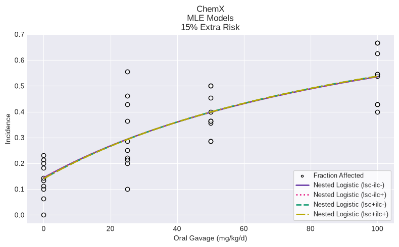
Multiple model fit (sessions) and model recommendation
A Session allows for multiple different models to be executed and potentially compared for model recommendation and selection.
A common pattern may be to add multiple versions of the same model with varying settings for the litter specific covariate and intralitter correlation. In the example below, we run instances of the Nested Logistic model, with different settings:
session = pybmds.Session(dataset=dataset)

for lsc in [LitterSpecificCovariate.Unused, LitterSpecificCovariate.OverallMean]:
    for ilc in [IntralitterCorrelation.Zero, IntralitterCorrelation.Estimate]:
        session.add_model(
            pybmds.Models.NestedLogistic,
            settings={
                "bmr": 0.15,
                "litter_specific_covariate": lsc,
                "intralitter_correlation": ilc,
            }
        )

session.execute()
fig = session.plot()
Model recommendation can be enabled, and if a recommendation is made, you can view outputs:
session.recommend()

if session.recommended_model is not None:
    fig = session.recommended_model.plot()
    print(session.recommended_model.text())
Nested Logistic (lsc-ilc-) Model
══════════════════════════════

Version: pybmds 25.2 (bmdscore 25.2)

Input Summary:
╒══════════════════════════════╤════════════════╕
│ BMR                          │ 15% Extra Risk │
│ Confidence Level (one sided) │ 0.95           │
│ Litter Specific Covariate    │ Unused         │
│ Intralitter Correlation      │ Zero           │
│ Estimate Background          │ True           │
│ Bootstrap Runs               │ 3              │
│ Bootstrap Iterations         │ 1000           │
│ Bootstrap Seed               │ 237            │
╘══════════════════════════════╧════════════════╛

Parameter Settings:
╒═════════════╤═══════════╤═══════╤════════╕
│ Parameter   │   Initial │   Min │    Max │
╞═════════════╪═══════════╪═══════╪════════╡
│ a           │         0 │     0 │  1     │
│ b           │         0 │   -18 │ 18     │
│ theta1      │         0 │     0 │  1     │
│ theta2      │         0 │   -18 │ 18     │
│ rho         │         1 │     1 │ 18     │
│ phi1        │         0 │     0 │  1e+06 │
│ phi2        │         0 │     0 │  1e+06 │
│ phi3        │         0 │     0 │  1e+06 │
│ phi4        │         0 │     0 │  1e+06 │
╘═════════════╧═══════════╧═══════╧════════╛

Modeling Summary:
╒════════════════╤═══════════╕
│ BMD            │   20.9591 │
│ BMDL           │   15.6043 │
│ BMDU           │   31.4387 │
│ AIC            │  545.311  │
│ P-Value        │    0.997  │
│ d.f.           │   36      │
│ Chi²           │   19.9391 │
│ Log-Likelihood │ -269.656  │
╘════════════════╧═══════════╛

Model Parameters:
╒════════════╤════════════╤════════════╤══════════════╕
│ Variable   │   Estimate │ On Bound   │ Std Error    │
╞════════════╪════════════╪════════════╪══════════════╡
│ a          │   0.144144 │ no         │ Not Reported │
│ b          │  -4.77717  │ no         │ Not Reported │
│ theta1     │   0        │ yes        │ Not Reported │
│ theta2     │   0        │ no         │ Not Reported │
│ rho        │   1        │ yes        │ Not Reported │
│ phi1       │   0        │ yes        │ Not Reported │
│ phi2       │   0        │ yes        │ Not Reported │
│ phi3       │   0        │ yes        │ Not Reported │
│ phi4       │   0        │ yes        │ Not Reported │
╘════════════╧════════════╧════════════╧══════════════╛
Standard errors estimates are not generated for parameters estimated on corresponding bounds,
although sampling error is present for all parameters, as a rule. Standard error estimates may not
be reliable as a basis for confidence intervals or tests when one or more parameters are on bounds.


Bootstrap Runs:
╒══════════╤═══════════╤═════════╤═════════╤═════════╤═════════╕
│ Run      │   P-Value │    50th │    90th │    95th │    99th │
╞══════════╪═══════════╪═════════╪═════════╪═════════╪═════════╡
│ 1        │     0.994 │ 38.3725 │ 50.371  │ 54.0309 │ 63.0062 │
│ 2        │     0.999 │ 38.713  │ 50.4982 │ 55.5581 │ 63.5534 │
│ 3        │     0.998 │ 39.1281 │ 51.7388 │ 55.6245 │ 62.3796 │
│ Combined │     0.997 │ 38.7032 │ 50.9967 │ 55.2243 │ 62.982  │
╘══════════╧═══════════╧═════════╧═════════╧═════════╧═════════╛

Scaled Residuals (for dose group nearest the BMD):
╒══════════════════════════════╤═══════════╕
│ Minimum scaled residual      │ -0.327053 │
│ Minimum ABS(scaled residual) │  0.327053 │
│ Average scaled residual      │ -0.327053 │
│ Average ABS(scaled residual) │  0.327053 │
│ Maximum scaled residual      │ -0.327053 │
│ Maximum ABS(scaled residual) │  0.327053 │
╘══════════════════════════════╧═══════════╛

Litter Data:
╒════════╤═══════╤══════════════╤════════════╤════════════╤════════════╤═══════════════════╕
│   Dose │   LSC │   Est. Prob. │   Litter N │   Expected │   Observed │   Scaled Residual │
╞════════╪═══════╪══════════════╪════════════╪════════════╪════════════╪═══════════════════╡
│      0 │     9 │     0.144144 │          9 │    1.29729 │          0 │        -1.23117   │
│      0 │     9 │     0.144144 │          9 │    1.29729 │          1 │        -0.28214   │
│      0 │    10 │     0.144144 │         10 │    1.44144 │          1 │        -0.397439  │
│      0 │    10 │     0.144144 │         10 │    1.44144 │          2 │         0.502892  │
│      0 │    11 │     0.144144 │         11 │    1.58558 │          2 │         0.355751  │
│      0 │    13 │     0.144144 │         13 │    1.87387 │          3 │         0.889241  │
│      0 │    14 │     0.144144 │         14 │    2.01801 │          2 │        -0.013705  │
│      0 │    14 │     0.144144 │         14 │    2.01801 │          3 │         0.747213  │
│      0 │    15 │     0.144144 │         15 │    2.16215 │          2 │        -0.119203  │
│      0 │    16 │     0.144144 │         16 │    2.3063  │          1 │        -0.929789  │
│     25 │     9 │     0.292969 │          9 │    2.63672 │          2 │        -0.466337  │
│     25 │     9 │     0.292969 │          9 │    2.63672 │          5 │         1.73086   │
│     25 │    10 │     0.292969 │         10 │    2.92969 │          1 │        -1.34078   │
│     25 │    10 │     0.292969 │         10 │    2.92969 │          2 │        -0.645966  │
│     25 │    11 │     0.292969 │         11 │    3.22266 │          4 │         0.514971  │
│     25 │    12 │     0.292969 │         12 │    3.51563 │          3 │        -0.327053  │
│     25 │    13 │     0.292969 │         13 │    3.8086  │          6 │         1.33543   │
│     25 │    14 │     0.292969 │         14 │    4.10157 │          3 │        -0.646871  │
│     25 │    14 │     0.292969 │         14 │    4.10157 │          4 │        -0.0596448 │
│     25 │    14 │     0.292969 │         14 │    4.10157 │          6 │         1.11481   │
│     50 │     7 │     0.397703 │          7 │    2.78392 │          2 │        -0.605396  │
│     50 │    10 │     0.397703 │         10 │    3.97703 │          5 │         0.660963  │
│     50 │    10 │     0.397703 │         10 │    3.97703 │          5 │         0.660963  │
│     50 │    11 │     0.397703 │         11 │    4.37474 │          4 │        -0.230857  │
│     50 │    11 │     0.397703 │         11 │    4.37474 │          4 │        -0.230857  │
│     50 │    11 │     0.397703 │         11 │    4.37474 │          4 │        -0.230857  │
│     50 │    11 │     0.397703 │         11 │    4.37474 │          5 │         0.385197  │
│     50 │    14 │     0.397703 │         14 │    5.56785 │          4 │        -0.856159  │
│     50 │    14 │     0.397703 │         14 │    5.56785 │          5 │        -0.310085  │
│     50 │    15 │     0.397703 │         15 │    5.96555 │          6 │         0.0181751 │
│    100 │     8 │     0.53536  │          8 │    4.28288 │          5 │         0.508356  │
│    100 │    10 │     0.53536  │         10 │    5.3536  │          4 │        -0.858238  │
│    100 │    11 │     0.53536  │         11 │    5.88896 │          6 │         0.0671306 │
│    100 │    11 │     0.53536  │         11 │    5.88896 │          6 │         0.0671306 │
│    100 │    12 │     0.53536  │         12 │    6.42431 │          8 │         0.912006  │
│    100 │    12 │     0.53536  │         12 │    6.42431 │          8 │         0.912006  │
│    100 │    13 │     0.53536  │         13 │    6.95967 │          7 │         0.0224248 │
│    100 │    14 │     0.53536  │         14 │    7.49503 │          6 │        -0.801135  │
│    100 │    14 │     0.53536  │         14 │    7.49503 │          6 │        -0.801135  │
╘════════╧═══════╧══════════════╧════════════╧════════════╧════════════╧═══════════════════╛
Select a best-fitting model
You may recommend a best fitting model based on a decision tree, but expert judgment is required for model selection.
You can select any model; in this example, we agree with the recommended model:
session.select(model=session.recommended_model, notes="Lowest AIC; recommended model")
Generated outputs (Excel, Word, JSON) would include model selection information.
Additional Nested Dichotomous Plottting
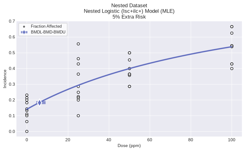
Some cases arise where models with intralitter correlation (ILC) estimated give a much better fit than corresponding models where ILC was not included in the model. This happens even when the estimated mean response rates (from the dose-response equation) appear very similar across those two models and very closely match the observations (as summarized in the traditional dose-response plots as the total number of responders over the total number of fetuses, ignoring litter membership).
For example, consider the following nested dichotomous data and modeling results:
import pybmds
import pandas as pd
from pybmds.models import nested_dichotomous
from pybmds.types.nested_dichotomous import LitterSpecificCovariate, IntralitterCorrelation

dataset = pybmds.NestedDichotomousDataset(
    name="Nested Dataset",
    dose_units="ppm",
    doses= [
        0, 0, 0, 0, 0, 0, 0, 0, 0, 0, 0, 0, 0, 0, 0, 0, 0, 0, 0, 0, 0, 0, 0,
        5, 5, 5, 5, 5, 5, 5, 5, 5, 5, 5, 5, 5, 5, 5, 5, 5, 5, 5, 5, 5, 5, 5, 5,
        15, 15, 15, 15, 15, 15, 15, 15, 15, 15, 15, 15, 15, 15, 15, 15, 15, 15, 15, 15, 15, 15, 15,
        25, 25, 25, 25, 25, 25, 25, 25, 25, 25, 25, 25, 25, 25, 25, 25, 25, 25, 25, 25, 25,
    ],
    litter_ns = [
        15, 15, 15, 12, 12, 16, 14, 13, 12, 16, 12, 14, 12, 15, 15, 16, 18, 14, 16, 17, 14, 9, 14,
        14, 14, 15, 7, 16, 12, 14, 14, 15, 16, 14, 15, 8, 15, 16, 14, 13, 17, 14, 17, 15, 14, 13, 16,
        15, 13, 14, 15, 14, 16, 16, 15, 15, 13, 15, 15, 15, 13, 14, 2, 16, 13, 17, 13, 16, 13, 17,
        13, 16, 15, 15, 12, 13, 16, 9, 11, 3, 7, 7, 13, 10, 13, 11, 17, 15, 13, 15, 13,
    ],
    incidences = [
        0, 2, 0, 2, 0, 0, 0, 1, 0, 2, 1, 0, 2, 0, 0, 6, 0, 1, 0, 0, 0, 3, 0,
        0, 0, 0, 0, 1, 0, 1, 1, 0, 0, 0, 1, 7, 0, 2, 0, 2, 0, 0, 0, 0, 1, 1, 1,
        0, 0, 0, 0, 1, 0, 12, 1, 1, 2, 0, 2, 1, 1, 5, 1, 6, 2, 0, 1, 1, 2, 0,
        13, 14, 15, 15, 12, 13, 16, 9, 11, 3, 7, 7, 13, 6, 13, 11, 17, 15, 13, 15, 13,
    ],
    litter_covariates = [
        15, 15, 15, 12, 12, 16, 14, 13, 12, 16, 12, 14, 12, 15, 15, 16, 18, 14, 16, 17, 14, 9, 14,
        14, 14, 15, 7, 16, 12, 14, 14, 15, 16, 14, 15, 8, 15, 16, 14, 13, 17, 14, 17, 15, 14, 13, 16,
        15, 13, 14, 15, 14, 16, 16, 15, 15, 13, 15, 15, 15, 13, 14, 2, 16, 13, 17, 13, 16, 13, 17,
        13, 16, 15, 15, 12, 13, 16, 9, 11, 3, 7, 7, 13, 10, 13, 11, 17, 15, 13, 15, 13,
    ]
)

# create a BMD session
session = pybmds.Session(dataset=dataset)

# add all combinations of litter specific covariate and intralitter correlation models
for lsc in [LitterSpecificCovariate.Unused, LitterSpecificCovariate.OverallMean]:
    for ilc in [IntralitterCorrelation.Zero, IntralitterCorrelation.Estimate]:
        session.add_model(
            pybmds.Models.NestedLogistic,
            settings={
                "bmr": 0.10,
                "litter_specific_covariate": lsc,
                "intralitter_correlation": ilc,
            }
        )

# execute the session
session.execute()

def summary_table(session):
    data = []
    for model in session.models:
        data.append([
            model.name(),
            model.results.bmdl,
            model.results.bmd,
            model.results.bmdu,
            model.results.combined_pvalue,
            model.results.aic
        ])

    df = pd.DataFrame(
        data=data,
        columns=["Model", "BMDL", "BMD", "BMDU", "P-Value", "AIC"]
    )
    return df

summary_table(session)
| Model | BMDL | BMD | BMDU | P-Value | AIC | |
|---|---|---|---|---|---|---|
| 0 | Nested Logistic (lsc-ilc-) | 12.572009 | 13.063484 | 15.240732 | 0.000000 | 665.740960 |
| 1 | Nested Logistic (lsc-ilc+) | 12.435465 | 13.576541 | 20.364812 | 0.459667 | 530.921493 |
| 2 | Nested Logistic (lsc+ilc-) | 13.067425 | 13.612183 | 20.418275 | 0.000000 | 624.327292 |
| 3 | Nested Logistic (lsc+ilc+) | 13.051740 | 14.221841 | 21.332762 | 0.576667 | 520.369276 |
Note that both models with ILC estimated (lsc+ilc+ and lsc-ilc=) both have p-values > 0.10 (indicating adequate fit) but that all variations of the nested logistic model have very similar BMD and BMDL values.
To show the fit for all models on a single plot:
fig1 = session.plot()
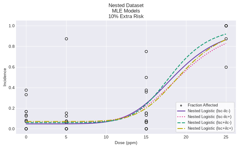
As can be seen above, all the variations of the nested logistic model appear to provide adequate fit to the observed responses. However, the traditional dose-response plots do not provide enough information to visually ascertain why certain variations of the nested logistic model do not statistically fit the observed data.
Therefore, for nested dichotomous data, there is another plot that can be generated that plots the observed number of litters with a certain number of responding fetuses and the model estimate of that value. Then, users can visually ascertain how well each variation of the nested logistic model predicts the “correct” observed number of litters with a particular number of responding fetuses.
from pybmds.plotting.nested_dichotomous import dose_litter_response_plot

fig = dose_litter_response_plot(session)
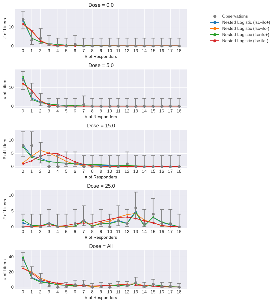
As can be seen above, at dose = 0 ppm, the models with ILC estimated (i.e., ilc+) clearly do a much better job at predicting the number of litters with 0 or 1 responding fetuses compared to models without ILC (i.e., ilc-). At dose = 5 ppm, the ilc+ and ilc- models continue to differ, but the differences in performance are less. However, at dose = 15 ppm, differences in model performance are stark with the ilc- models failing to predict accurately the the number of litters with 0 - 5 responding fetuses. The failure of the ilc- models in this dose group are most severe and may contribute the most to these models having poor statistical fit to the observed data (as indicated by the very low p-values).
Rao-Scott Transformation for Summary Level Data
Running the nested dichotomous models requires individual level data (i.e., fetal incidence data for each individual dam in each dose group in the dataset). However, it is often the case that individual level data is not available and only fetal summary data (i.e., fetal incidence data per dose group, irrespective of litter membership) is reported. The Rao-Scott transformation, described in Fox et al., 2017, is an approach that scales dose-level fetal incidence and sample size data by a variable called the design effect in order to approximate the intralitter correlation that occurs due the clustered study design of development toxicity studies (see BMDS User Guide for complete details).
Consider a regular dichotomous dataset saved as a CSV file:
import pybmds
import pandas as pd

df = pd.read_csv('data/example-rao-scott.csv')
df
| dose | n | incidence | |
|---|---|---|---|
| 0 | 0 | 470 | 11 |
| 1 | 7 | 211 | 6 |
| 2 | 35 | 232 | 2 |
| 3 | 100 | 220 | 7 |
| 4 | 175 | 241 | 14 |
| 5 | 350 | 237 | 39 |
| 6 | 500 | 166 | 57 |
The Rao-Scott transformation can be run by defining your dataset as the loaded CSV file and then calling RaoScott class. Note that the only user input necessary is to define the species used in the toxicity study; the Rao-Scott transformation is currently available for studies conducted with rats, mice, or rabbits.
from pybmds.datasets.transforms.rao_scott import RaoScott

# Example data
dataset= pybmds.DichotomousDataset(
    doses = df["dose"].tolist(),
    ns = df["n"].tolist(),
    incidences = df["incidence"].tolist(),
    name = "Example Rao-Scott",
    dose_units="mg/kg",
)

# Now run the Rao-Scott transformation
rs = RaoScott(
    dataset = dataset,
    species="rat",
)

display(rs.summary_df())
fig = rs.figure()
| Dose | N | Incidence | Fraction Affected | Design Effect (LS) | Design Effect (OR) | Design Effect (Average) | N (Rao-Scott Transformed) | Incidence (Rao-Scott Transformed) | |
|---|---|---|---|---|---|---|---|---|---|
| 0 | 0 | 470 | 11 | 0.023404 | 1.656569 | 1.651469 | 1.654019 | 284.156347 | 6.650468 |
| 1 | 7 | 211 | 6 | 0.028436 | 1.766866 | 1.774509 | 1.770687 | 119.162766 | 3.388515 |
| 2 | 35 | 232 | 2 | 0.008621 | 1.190248 | 1.142393 | 1.166320 | 198.916165 | 1.714795 |
| 3 | 100 | 220 | 7 | 0.031818 | 1.833828 | 1.849642 | 1.841735 | 119.452574 | 3.800764 |
| 4 | 175 | 241 | 14 | 0.058091 | 2.238174 | 2.309710 | 2.273942 | 105.983357 | 6.156710 |
| 5 | 350 | 237 | 39 | 0.164557 | 3.159175 | 3.391730 | 3.275453 | 72.356414 | 11.906752 |
| 6 | 500 | 166 | 57 | 0.343373 | 4.030063 | 4.449370 | 4.239716 | 39.153563 | 13.444296 |
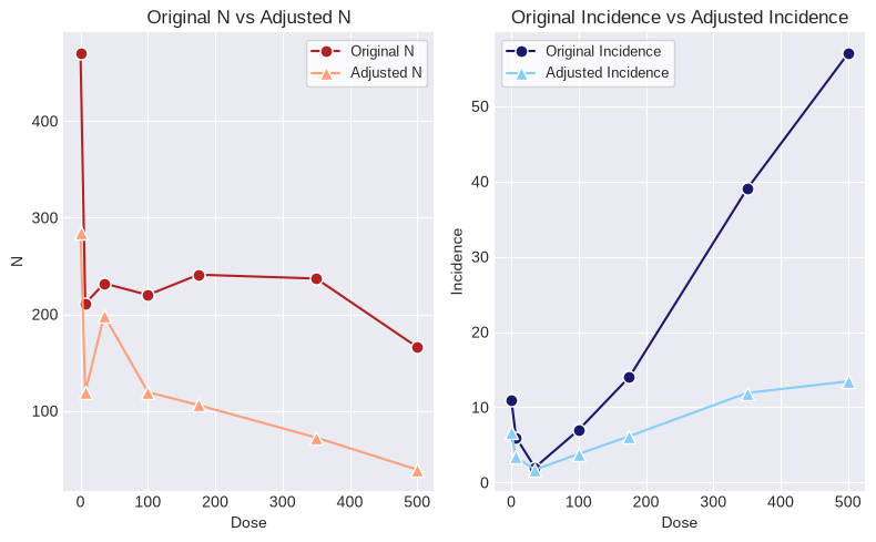
The Rao-Scott transformed Ns and incidence values can now be used in a Dichotomous analysis and the resulting BMD, BMDL, and BMDU will reflect the increased variance introduced into the modeling by scaling the N and incidence values.