Dichotomous Data
Table of Contents
Quickstart
To run a dichotomous dataset:
import pybmds
dataset = pybmds.DichotomousDataset(
doses=[0, 25, 75, 125, 200],
ns=[20, 20, 20, 20, 20],
incidences=[0, 1, 7, 15, 19],
)
# create a BMD session
session = pybmds.Session(dataset=dataset)
# add all default models
session.add_default_models()
# execute the session
session.execute()
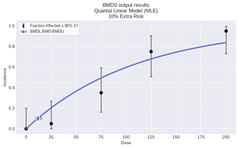
# recommend a best-fitting model
session.recommend()
if session.recommended_model is not None:
fig = session.recommended_model.plot()
print(session.recommended_model.text())
# save excel report
df = session.to_df()
df.to_excel("output/report.xlsx")
# save to a word report
report = session.to_docx()
report.save("output/report.docx")
     Quantal Linear Model
══════════════════════════════

Version: pybmds 25.2 (bmdscore 25.2)

Input Summary:
╒══════════════════════════════╤══════════════════════════╕
│ BMR                          │ 10% Extra Risk           │
│ Confidence Level (one sided) │ 0.95                     │
│ Modeling approach            │ frequentist_unrestricted │
╘══════════════════════════════╧══════════════════════════╛

Parameter Settings:
╒═════════════╤═══════════╤═══════╤═══════╕
│ Parameter   │   Initial │   Min │   Max │
╞═════════════╪═══════════╪═══════╪═══════╡
│ g           │         0 │   -18 │    18 │
│ b           │         0 │     0 │   100 │
╘═════════════╧═══════════╧═══════╧═══════╛

Modeling Summary:
╒════════════════╤════════════╕
│ BMD            │  11.6404   │
│ BMDL           │   8.91584  │
│ BMDU           │  15.4669   │
│ AIC            │  74.7575   │
│ Log-Likelihood │ -36.3787   │
│ P-Value        │   0.142335 │
│ Overall d.f.   │   4        │
│ Chi²           │   6.88058  │
╘════════════════╧════════════╛

Model Parameters:
╒════════════╤════════════╤════════════╤══════════════╕
│ Variable   │   Estimate │ On Bound   │ Std Error    │
╞════════════╪════════════╪════════════╪══════════════╡
│ g          │ 1.523e-08  │ yes        │ Not Reported │
│ b          │ 0.00905126 │ no         │ 0.0015129    │
╘════════════╧════════════╧════════════╧══════════════╛
Standard errors estimates are not generated for parameters estimated on corresponding bounds,
although sampling error is present for all parameters, as a rule. Standard error estimates may not
be reliable as a basis for confidence intervals or tests when one or more parameters are on bounds.


Goodness of Fit:
╒════════╤════════╤════════════╤════════════╤════════════╤═══════════════════╕
│   Dose │   Size │   Observed │   Expected │   Est Prob │   Scaled Residual │
╞════════╪════════╪════════════╪════════════╪════════════╪═══════════════════╡
│      0 │     20 │          0 │  3.046e-07 │  1.523e-08 │      -0.000551905 │
│     25 │     20 │          1 │  4.05013   │  0.202506  │      -1.69715     │
│     75 │     20 │          7 │  9.85595   │  0.492797  │      -1.27735     │
│    125 │     20 │         15 │ 13.5484    │  0.677421  │       0.694349    │
│    200 │     20 │         19 │ 16.7277    │  0.836387  │       1.3735      │
╘════════╧════════╧════════════╧════════════╧════════════╧═══════════════════╛

Analysis of Deviance:
╒═══════════════╤══════════════════╤════════════╤════════════╤═════════════╤═════════════╕
│ Model         │   Log-Likelihood │   # Params │ Deviance   │ Test d.f.   │ P-Value     │
╞═══════════════╪══════════════════╪════════════╪════════════╪═════════════╪═════════════╡
│ Full model    │         -32.1362 │          5 │ -          │ -           │ -           │
│ Fitted model  │         -36.3787 │          1 │ 8.485      │ 4           │ 0.0753431   │
│ Reduced model │         -68.0292 │          1 │ 71.7859    │ 4           │ 9.54792e-15 │
╘═══════════════╧══════════════════╧════════════╧════════════╧═════════════╧═════════════╛
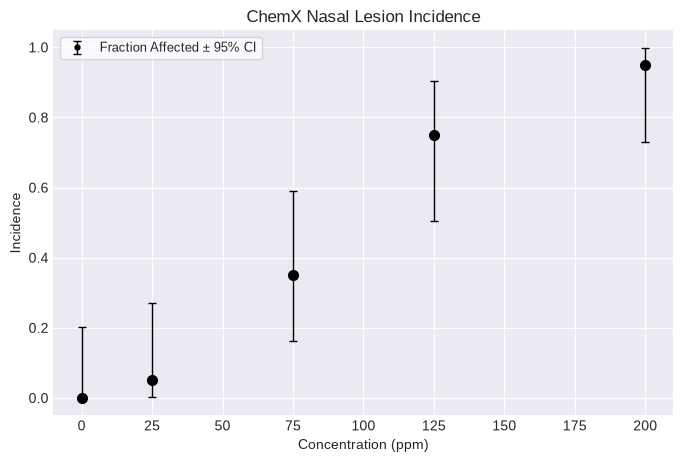
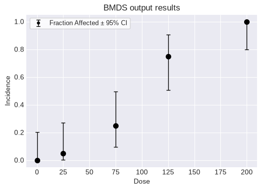
Dichotomous datasets
Creating a dichotomous dataset requires a list of doses, incidences, and the total number of subjects, one item per dose group. Doses must be unique.
You can also add optional attributes, such as name, dose_name, dose_units, response_name, response_units, etc.
For example:
dataset = pybmds.DichotomousDataset(
    name="ChemX Nasal Lesion Incidence",
    dose_name="Concentration",
    dose_units="ppm",
    doses=[0, 25, 75, 125, 200],
    ns=[20, 20, 20, 20, 20],
    incidences=[0, 1, 7, 15, 19],
)

fig = dataset.plot()
Single model fit
You can fit a specific model to the dataset and plot/print the results. The printed results will include the BMD, BMDL, BMDU, p-value, AIC, etc.
The individual models available are shown below. Note that the degrees of the Multistage model can be increased to a maximum of the lesser of N-1 or 8 (as specified in the BMDS User Guide).
from pybmds.models import dichotomous
dichotomous.QuantalLinear(dataset)
dichotomous.Multistage(dataset, settings={"degree": 2})
dichotomous.Multistage(dataset, settings={"degree": 3})
dichotomous.Logistic(dataset)
dichotomous.LogLogistic(dataset)
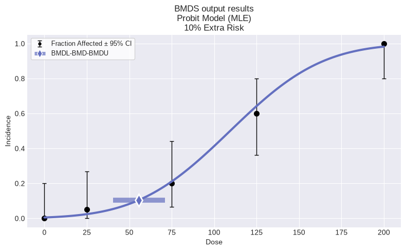
dichotomous.Probit(dataset)
dichotomous.LogProbit(dataset)
dichotomous.Gamma(dataset)
dichotomous.Weibull(dataset)
dichotomous.DichotomousHill(dataset)
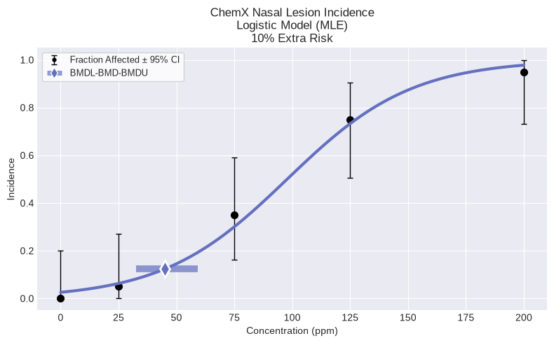
As an example, to fit the Logistic model:
model = dichotomous.Logistic(dataset)
model.execute()
fig = model.plot()
To generate an output report:
print(model.text())
        Logistic Model
══════════════════════════════

Version: pybmds 25.2 (bmdscore 25.2)

Input Summary:
╒══════════════════════════════╤══════════════════════════╕
│ BMR                          │ 10% Extra Risk           │
│ Confidence Level (one sided) │ 0.95                     │
│ Modeling approach            │ frequentist_unrestricted │
╘══════════════════════════════╧══════════════════════════╛

Parameter Settings:
╒═════════════╤═══════════╤═══════╤═══════╕
│ Parameter   │   Initial │   Min │   Max │
╞═════════════╪═══════════╪═══════╪═══════╡
│ a           │         0 │   -18 │    18 │
│ b           │         0 │     0 │   100 │
╘═════════════╧═══════════╧═══════╧═══════╛

Modeling Summary:
╒════════════════╤════════════╕
│ BMD            │  44.8841   │
│ BMDL           │  32.5885   │
│ BMDU           │  59.2      │
│ AIC            │  70.1755   │
│ Log-Likelihood │ -33.0878   │
│ P-Value        │   0.666151 │
│ Overall d.f.   │   3        │
│ Chi²           │   1.57027  │
╘════════════════╧════════════╛

Model Parameters:
╒════════════╤════════════╤════════════╤═════════════╕
│ Variable   │   Estimate │ On Bound   │   Std Error │
╞════════════╪════════════╪════════════╪═════════════╡
│ a          │ -3.62365   │ no         │  0.707213   │
│ b          │  0.0370501 │ no         │  0.00705474 │
╘════════════╧════════════╧════════════╧═════════════╛

Goodness of Fit:
╒════════╤════════╤════════════╤════════════╤════════════╤═══════════════════╕
│   Dose │   Size │   Observed │   Expected │   Est Prob │   Scaled Residual │
╞════════╪════════╪════════════╪════════════╪════════════╪═══════════════════╡
│      0 │     20 │          0 │    0.51983 │  0.0259915 │         -0.730549 │
│     25 │     20 │          1 │    1.26254 │  0.063127  │         -0.241397 │
│     75 │     20 │          7 │    6.01009 │  0.300505  │          0.482793 │
│    125 │     20 │         15 │   14.651   │  0.732552  │          0.176289 │
│    200 │     20 │         19 │   19.5565  │  0.977825  │         -0.845059 │
╘════════╧════════╧════════════╧════════════╧════════════╧═══════════════════╛

Analysis of Deviance:
╒═══════════════╤══════════════════╤════════════╤════════════╤═════════════╤═════════════╕
│ Model         │   Log-Likelihood │   # Params │ Deviance   │ Test d.f.   │ P-Value     │
╞═══════════════╪══════════════════╪════════════╪════════════╪═════════════╪═════════════╡
│ Full model    │         -32.1362 │          5 │ -          │ -           │ -           │
│ Fitted model  │         -33.0878 │          2 │ 1.90305    │ 3           │ 0.592771    │
│ Reduced model │         -68.0292 │          1 │ 71.7859    │ 4           │ 9.54792e-15 │
╘═══════════════╧══════════════════╧════════════╧════════════╧═════════════╧═════════════╛
Change input settings
The default settings use a BMR of 10% Extra Risk and a 95% confidence interval. If you fit a single model to your dataset, settings for that model can be modified:
model = dichotomous.Logistic(
    dataset, settings={"bmr": 0.15, "bmr_type": pybmds.DichotomousRiskType.AddedRisk}
)
print(model.settings.tbl())
╒══════════════════════════════╤══════════════════════════╕
│ BMR                          │ 15% Added Risk           │
│ Confidence Level (one sided) │ 0.95                     │
│ Modeling approach            │ frequentist_unrestricted │
│ Degree                       │ 0                        │
╘══════════════════════════════╧══════════════════════════╛
Change parameter settings
If you want to see a preview of the initial parameter settings, you can run:
model = dichotomous.Logistic(dataset)
print(model.priors_tbl())
╒═════════════╤═══════════╤═══════╤═══════╕
│ Parameter   │   Initial │   Min │   Max │
╞═════════════╪═══════════╪═══════╪═══════╡
│ a           │         0 │   -18 │    18 │
│ b           │         0 │     0 │   100 │
╘═════════════╧═══════════╧═══════╧═══════╛
You can also change the initial parameter settings shown above for any run of a single dichotomous model.
Continuing with the Logistic model example, for the a parameter, you can change the minimum and maximum range from -10 to 10, while b can range from 0 to 50:
model.settings.priors.update("a", min_value=-10, max_value=10)
model.settings.priors.update("b", min_value=0, max_value=50)
print(model.priors_tbl())
╒═════════════╤═══════════╤═══════╤═══════╕
│ Parameter   │   Initial │   Min │   Max │
╞═════════════╪═══════════╪═══════╪═══════╡
│ a           │         0 │   -10 │    10 │
│ b           │         0 │     0 │    50 │
╘═════════════╧═══════════╧═══════╧═══════╛
You can change the range and initial value for any parameter in the model by following the same steps above.
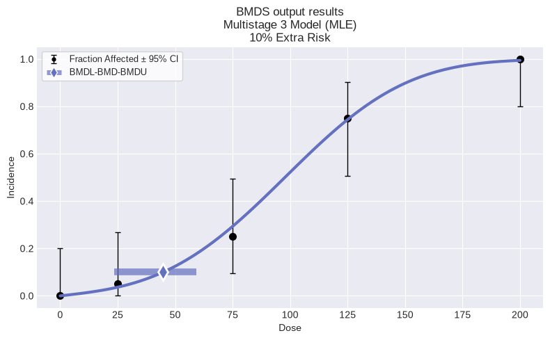
Multiple model fit (sessions) and model recommendation
To run all the default models, save the results, and save the plot of the fit of the recommended model with the data:
dataset = pybmds.DichotomousDataset(
    doses=[0, 25, 75, 125, 200],
    ns=[20, 20, 20, 20, 20],
    incidences=[0, 1, 7, 15, 19],
)

# create a BMD session
session = pybmds.Session(dataset=dataset)

# add all default models
session.add_default_models()

# execute the session
session.execute()

# recommend a best-fitting model
session.recommend()

# print recommended model and plot recommended model with dataset
model_index = session.recommender.results.recommended_model_index
if model_index:
    model = session.models[model_index]
    display(model.plot())
    print(model.text())
     Quantal Linear Model
══════════════════════════════

Version: pybmds 25.2 (bmdscore 25.2)

Input Summary:
╒══════════════════════════════╤══════════════════════════╕
│ BMR                          │ 10% Extra Risk           │
│ Confidence Level (one sided) │ 0.95                     │
│ Modeling approach            │ frequentist_unrestricted │
╘══════════════════════════════╧══════════════════════════╛

Parameter Settings:
╒═════════════╤═══════════╤═══════╤═══════╕
│ Parameter   │   Initial │   Min │   Max │
╞═════════════╪═══════════╪═══════╪═══════╡
│ g           │         0 │   -18 │    18 │
│ b           │         0 │     0 │   100 │
╘═════════════╧═══════════╧═══════╧═══════╛

Modeling Summary:
╒════════════════╤════════════╕
│ BMD            │  11.6404   │
│ BMDL           │   8.91584  │
│ BMDU           │  15.4669   │
│ AIC            │  74.7575   │
│ Log-Likelihood │ -36.3787   │
│ P-Value        │   0.142335 │
│ Overall d.f.   │   4        │
│ Chi²           │   6.88058  │
╘════════════════╧════════════╛

Model Parameters:
╒════════════╤════════════╤════════════╤══════════════╕
│ Variable   │   Estimate │ On Bound   │ Std Error    │
╞════════════╪════════════╪════════════╪══════════════╡
│ g          │ 1.523e-08  │ yes        │ Not Reported │
│ b          │ 0.00905126 │ no         │ 0.0015129    │
╘════════════╧════════════╧════════════╧══════════════╛
Standard errors estimates are not generated for parameters estimated on corresponding bounds,
although sampling error is present for all parameters, as a rule. Standard error estimates may not
be reliable as a basis for confidence intervals or tests when one or more parameters are on bounds.


Goodness of Fit:
╒════════╤════════╤════════════╤════════════╤════════════╤═══════════════════╕
│   Dose │   Size │   Observed │   Expected │   Est Prob │   Scaled Residual │
╞════════╪════════╪════════════╪════════════╪════════════╪═══════════════════╡
│      0 │     20 │          0 │  3.046e-07 │  1.523e-08 │      -0.000551905 │
│     25 │     20 │          1 │  4.05013   │  0.202506  │      -1.69715     │
│     75 │     20 │          7 │  9.85595   │  0.492797  │      -1.27735     │
│    125 │     20 │         15 │ 13.5484    │  0.677421  │       0.694349    │
│    200 │     20 │         19 │ 16.7277    │  0.836387  │       1.3735      │
╘════════╧════════╧════════════╧════════════╧════════════╧═══════════════════╛

Analysis of Deviance:
╒═══════════════╤══════════════════╤════════════╤════════════╤═════════════╤═════════════╕
│ Model         │   Log-Likelihood │   # Params │ Deviance   │ Test d.f.   │ P-Value     │
╞═══════════════╪══════════════════╪════════════╪════════════╪═════════════╪═════════════╡
│ Full model    │         -32.1362 │          5 │ -          │ -           │ -           │
│ Fitted model  │         -36.3787 │          1 │ 8.485      │ 4           │ 0.0753431   │
│ Reduced model │         -68.0292 │          1 │ 71.7859    │ 4           │ 9.54792e-15 │
╘═══════════════╧══════════════════╧════════════╧════════════╧═════════════╧═════════════╛
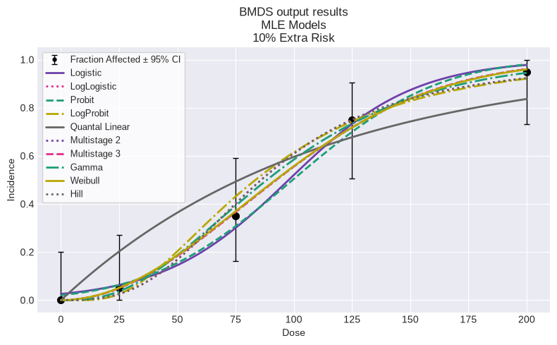
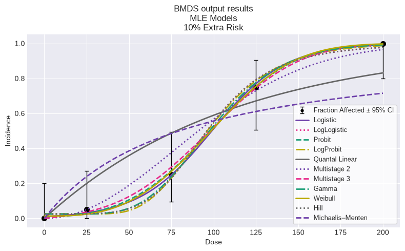
You can also plot all models:
fig = session.plot()
To print a summary table of modeling results, create a custom function:
import pandas as pd

def summary_table(session):
    data = []
    for model in session.models:
        data.append([
            model.name(),
            model.results.bmdl,
            model.results.bmd,
            model.results.bmdu,
            model.results.gof.p_value,
            model.results.fit.aic
        ])

    df = pd.DataFrame(
        data=data,
        columns=["Model", "BMDL", "BMD", "BMDU", "P-Value", "AIC"]
    )
    return df

summary_table(session)
| Model | BMDL | BMD | BMDU | P-Value | AIC | |
|---|---|---|---|---|---|---|
| 0 | Logistic | 32.588454 | 44.884135 | 59.199959 | 0.666151 | 70.175538 |
| 1 | LogLogistic | 25.629773 | 40.699410 | 55.230166 | 0.828331 | 69.093671 |
| 2 | Probit | 30.363157 | 41.862869 | 55.948994 | 0.604658 | 70.259470 |
| 3 | LogProbit | 24.847658 | 37.801377 | 50.504284 | 0.741253 | 69.462536 |
| 4 | Quantal Linear | 8.915836 | 11.640424 | 15.466867 | 0.142335 | 74.757493 |
| 5 | Multistage 2 | 18.233585 | 35.929912 | 42.102724 | 0.979879 | 68.456130 |
| 6 | Multistage 3 | 16.215191 | 35.929433 | 50.620322 | 0.979879 | 68.456130 |
| 7 | Gamma | 22.220274 | 37.500667 | 51.773296 | 0.963613 | 68.546957 |
| 8 | Weibull | 20.810667 | 35.515406 | 50.622612 | 0.980762 | 68.452316 |
| 9 | Hill | 25.629773 | 40.699410 | 55.230167 | 0.828331 | 69.093671 |
To generate Excel and Word reports:
# save excel report
df = session.to_df()
df.to_excel("output/report.xlsx")

# save to a word report
report = session.to_docx()
report.save("output/report.docx")
Change session settings
If you run all the default models and select the best fit, you can change these settings by:
session.add_default_models(
    settings={
        "bmr": 0.15,
        "bmr_type": pybmds.DichotomousRiskType.AddedRisk,
        "alpha": 0.1
    }
)
This would run the dichotomous models for a BMR of 15% Added Risk at a 90% confidence interval.
Run subset of models
You can select a set of models, rather than using all available models.
For example, to evaluate the Logistic, Probit, Quantal Linear, and Weibull models:
session = pybmds.Session(dataset=dataset)
session.add_model(pybmds.Models.Weibull)
session.add_model(pybmds.Models.Logistic)
session.add_model(pybmds.Models.Probit)
session.add_model(pybmds.Models.QuantalLinear)

session.execute()
Custom models
You can run a session with custom models where the model name has been changed, initial parameter values have been modified and parameter values have been set to a particular value.
We start with a new dataset:
dataset = pybmds.DichotomousDataset(
    doses=[0, 25, 75, 125, 200],
    ns=[20, 20, 20, 20, 20],
    incidences=[0, 1, 5, 15, 20],
)
fig = dataset.plot(figsize=(6,4))
And add this dataset to a new modeling session, along with all the standard models:
# create a BMD session
session = pybmds.Session(dataset=dataset)

# add all default models
session.add_default_models()
Next, add a modified Dichotomous Hill model with the slope parameter fixed to 1, resulting in the Michaelis-Menten model:
model = pybmds.models.dichotomous.DichotomousHill(dataset, settings={"name": "Michaelis–Menten"})

# fix the `b` parameter to 1
model.settings.priors.update("b", initial_value=1, min_value=1, max_value=1)

session.models.append(model)
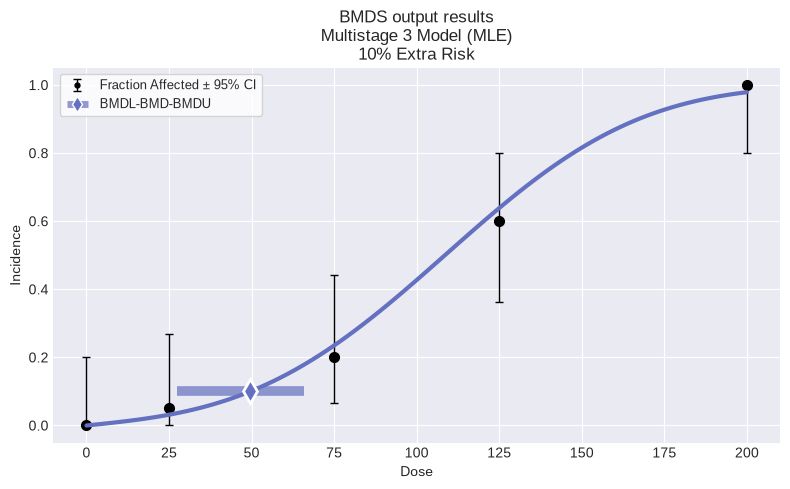
To run the default models and any manually added models, save the results, and save the plot of the fitted recommended model with the data:
# execute the session
session.execute()

# recommend a best-fitting model
session.recommend()

# print recommended model and plot recommended model with dataset
model_index = session.recommender.results.recommended_model_index
if model_index:
    model = session.models[model_index]
    display(model.plot())
    print(model.text())
      Multistage 3 Model
══════════════════════════════

Version: pybmds 25.2 (bmdscore 25.2)

Input Summary:
╒══════════════════════════════╤════════════════════════╕
│ BMR                          │ 10% Extra Risk         │
│ Confidence Level (one sided) │ 0.95                   │
│ Modeling approach            │ frequentist_restricted │
│ Degree                       │ 3                      │
╘══════════════════════════════╧════════════════════════╛

Parameter Settings:
╒═════════════╤═══════════╤═══════╤═══════╕
│ Parameter   │   Initial │   Min │   Max │
╞═════════════╪═══════════╪═══════╪═══════╡
│ g           │         0 │   -18 │    18 │
│ b1          │         0 │     0 │ 10000 │
│ b2          │         0 │     0 │ 10000 │
│ b3          │         0 │     0 │ 10000 │
╘═════════════╧═══════════╧═══════╧═══════╛

Modeling Summary:
╒════════════════╤════════════╕
│ BMD            │  44.7215   │
│ BMDL           │  23.5185   │
│ BMDU           │  59.29     │
│ AIC            │  55.4222   │
│ Log-Likelihood │ -26.7111   │
│ P-Value        │   0.982997 │
│ Overall d.f.   │   4        │
│ Chi²           │   0.393601 │
╘════════════════╧════════════╛

Model Parameters:
╒════════════╤═════════════╤════════════╤══════════════╕
│ Variable   │    Estimate │ On Bound   │ Std Error    │
╞════════════╪═════════════╪════════════╪══════════════╡
│ g          │ 1.523e-08   │ yes        │ Not Reported │
│ b1         │ 0.00109945  │ no         │ 0.282148     │
│ b2         │ 1.3118e-20  │ yes        │ Not Reported │
│ b3         │ 6.28232e-07 │ yes        │ Not Reported │
╘════════════╧═════════════╧════════════╧══════════════╛
Standard errors estimates are not generated for parameters estimated on corresponding bounds,
although sampling error is present for all parameters, as a rule. Standard error estimates may not
be reliable as a basis for confidence intervals or tests when one or more parameters are on bounds.


Goodness of Fit:
╒════════╤════════╤════════════╤════════════╤════════════╤═══════════════════╕
│   Dose │   Size │   Observed │   Expected │   Est Prob │   Scaled Residual │
╞════════╪════════╪════════════╪════════════╪════════════╪═══════════════════╡
│      0 │     20 │          0 │  3.046e-07 │  1.523e-08 │      -0.000551905 │
│     25 │     20 │          1 │  0.732306  │  0.0366153 │       0.318708    │
│     75 │     20 │          5 │  5.87088   │  0.293544  │      -0.427626    │
│    125 │     20 │         15 │ 14.8896    │  0.744478  │       0.0566184   │
│    200 │     20 │         20 │ 19.8946    │  0.99473   │       0.325509    │
╘════════╧════════╧════════════╧════════════╧════════════╧═══════════════════╛

Analysis of Deviance:
╒═══════════════╤══════════════════╤════════════╤════════════╤═════════════╤═══════════╕
│ Model         │   Log-Likelihood │   # Params │ Deviance   │ Test d.f.   │ P-Value   │
╞═══════════════╪══════════════════╪════════════╪════════════╪═════════════╪═══════════╡
│ Full model    │         -26.4637 │          5 │ -          │ -           │ -         │
│ Fitted model  │         -26.7111 │          1 │ 0.494739   │ 4           │ 0.974011  │
│ Reduced model │         -67.6859 │          1 │ 82.4443    │ 4           │ 0         │
╘═══════════════╧══════════════════╧════════════╧════════════╧═════════════╧═══════════╛
You can also plot all models on a single plot:
fig = session.plot()
We can summarize using the summary_table function we defined above:
summary_table(session)
| Model | BMDL | BMD | BMDU | P-Value | AIC | |
|---|---|---|---|---|---|---|
| 0 | Logistic | 38.978523 | 53.621709 | 68.574734 | 0.882992 | 57.937669 |
| 1 | LogLogistic | 42.571336 | 63.282243 | 79.375096 | 0.425015 | 61.482744 |
| 2 | Probit | 35.679901 | 49.803548 | 64.425011 | 0.904740 | 57.636693 |
| 3 | LogProbit | 46.554482 | 64.255617 | 78.221184 | 0.482500 | 61.039679 |
| 4 | Quantal Linear | 9.034209 | 11.838419 | 15.792424 | 0.018000 | 71.369122 |
| 5 | Multistage 2 | 23.966481 | 35.476547 | 41.646639 | 0.714606 | 57.828036 |
| 6 | Multistage 3 | 23.518491 | 44.721502 | 59.289977 | 0.982997 | 55.422160 |
| 7 | Gamma | 35.295248 | 62.094483 | 77.958640 | 0.531844 | 60.742566 |
| 8 | Weibull | 31.655618 | 53.126127 | 76.403822 | 0.815826 | 58.068448 |
| 9 | Hill | 42.537341 | 63.282242 | 79.375096 | 0.425015 | 61.482745 |
| 10 | Michaelis–Menten | 6.000057 | 8.848340 | 9.676710 | 0.001267 | 80.014221 |
Model recommendation and selection
The pybmds package may recommend a best-fitting model based on a decision tree, but expert judgment may be required for model selection. To run model recommendation and view a recommended model, if one is recommended:
session.recommend()

if session.recommended_model is not None:
    display(session.recommended_model.plot())
    print(session.recommended_model.text())
      Multistage 3 Model
══════════════════════════════

Version: pybmds 25.2 (bmdscore 25.2)

Input Summary:
╒══════════════════════════════╤════════════════════════╕
│ BMR                          │ 10% Extra Risk         │
│ Confidence Level (one sided) │ 0.95                   │
│ Modeling approach            │ frequentist_restricted │
│ Degree                       │ 3                      │
╘══════════════════════════════╧════════════════════════╛

Parameter Settings:
╒═════════════╤═══════════╤═══════╤═══════╕
│ Parameter   │   Initial │   Min │   Max │
╞═════════════╪═══════════╪═══════╪═══════╡
│ g           │         0 │   -18 │    18 │
│ b1          │         0 │     0 │ 10000 │
│ b2          │         0 │     0 │ 10000 │
│ b3          │         0 │     0 │ 10000 │
╘═════════════╧═══════════╧═══════╧═══════╛

Modeling Summary:
╒════════════════╤════════════╕
│ BMD            │  44.7215   │
│ BMDL           │  23.5185   │
│ BMDU           │  59.29     │
│ AIC            │  55.4222   │
│ Log-Likelihood │ -26.7111   │
│ P-Value        │   0.982997 │
│ Overall d.f.   │   4        │
│ Chi²           │   0.393601 │
╘════════════════╧════════════╛

Model Parameters:
╒════════════╤═════════════╤════════════╤══════════════╕
│ Variable   │    Estimate │ On Bound   │ Std Error    │
╞════════════╪═════════════╪════════════╪══════════════╡
│ g          │ 1.523e-08   │ yes        │ Not Reported │
│ b1         │ 0.00109945  │ no         │ 0.282148     │
│ b2         │ 1.3118e-20  │ yes        │ Not Reported │
│ b3         │ 6.28232e-07 │ yes        │ Not Reported │
╘════════════╧═════════════╧════════════╧══════════════╛
Standard errors estimates are not generated for parameters estimated on corresponding bounds,
although sampling error is present for all parameters, as a rule. Standard error estimates may not
be reliable as a basis for confidence intervals or tests when one or more parameters are on bounds.


Goodness of Fit:
╒════════╤════════╤════════════╤════════════╤════════════╤═══════════════════╕
│   Dose │   Size │   Observed │   Expected │   Est Prob │   Scaled Residual │
╞════════╪════════╪════════════╪════════════╪════════════╪═══════════════════╡
│      0 │     20 │          0 │  3.046e-07 │  1.523e-08 │      -0.000551905 │
│     25 │     20 │          1 │  0.732306  │  0.0366153 │       0.318708    │
│     75 │     20 │          5 │  5.87088   │  0.293544  │      -0.427626    │
│    125 │     20 │         15 │ 14.8896    │  0.744478  │       0.0566184   │
│    200 │     20 │         20 │ 19.8946    │  0.99473   │       0.325509    │
╘════════╧════════╧════════════╧════════════╧════════════╧═══════════════════╛

Analysis of Deviance:
╒═══════════════╤══════════════════╤════════════╤════════════╤═════════════╤═══════════╕
│ Model         │   Log-Likelihood │   # Params │ Deviance   │ Test d.f.   │ P-Value   │
╞═══════════════╪══════════════════╪════════════╪════════════╪═════════════╪═══════════╡
│ Full model    │         -26.4637 │          5 │ -          │ -           │ -         │
│ Fitted model  │         -26.7111 │          1 │ 0.494739   │ 4           │ 0.974011  │
│ Reduced model │         -67.6859 │          1 │ 82.4443    │ 4           │ 0         │
╘═══════════════╧══════════════════╧════════════╧════════════╧═════════════╧═══════════╛
You can select a best-fitting model and output reports generated will indicate this selection. This is a manual action. The example below selects the recommended model, but any model in the session could be selected.
session.select(model=session.recommended_model, notes="Lowest BMDL; recommended model")
Generated outputs (Excel, Word, JSON) would include model selection information.
Changing how parameters are counted
For the purposes of statistical calculations, e.g., calcuation the AIC value and p-values, BMDS only counts the number of parameters off their respective boundaries by default. But users have the option of parameterizing BMDS so that it counts all the parameters in a model, irrespective if they were estimated on or off of their boundaries.
Parameterizing BMDS to count all parameters will impact AIC and p-value calculations and therefore may impact the selection of models using the automatic model selection logic. For example, consider the following dataset run using the default setting of only counting parameters that are off a boundary.
import pybmds
import pandas as pd

dataset = pybmds.DichotomousDataset(
    doses=[0, 25, 75, 125, 200],
    ns=[20, 20, 20, 20, 20],
    incidences=[0, 1, 4, 12, 20],
)

# create a BMD session
session = pybmds.Session(dataset=dataset)

# add all default models
session.add_default_models()

# execute the session
session.execute()

# recommend a best-fitting model
session.recommend()

# Print out a summary table for the recommended model

model = session.recommended_model
if model is not None:
    df = pd.DataFrame([[
        model.name(),
        model.results.bmdl,
        model.results.bmd,
        model.results.bmdu,
        model.results.gof.test_statistic,
        model.results.gof.df,
        model.results.gof.p_value,
        model.results.fit.aic
    ]], columns=["Model", "BMDL", "BMD", "BMDU", "Chi2 statistic", "DF", "P-Value", "AIC"])
    df = df.T  # Transpose for vertical display
    df.columns = ["Value"]
    display(df)
else:
    print("No recommended model.")

fig = session.recommended_model.plot()
| Value | |
|---|---|
| Model | Multistage 3 |
| BMDL | 27.533975 |
| BMD | 49.575782 |
| BMDU | 66.008838 |
| Chi2 statistic | 0.917661 |
| DF | 4.0 |
| P-Value | 0.922014 |
| AIC | 58.188143 |
So, for this dataset, we can see that the automated model selection workflow chose the Multistage 3 model. We can also summarize the modeling results for all models in the session by using the summary_table function defined above:
summary_table(session)
| Model | BMDL | BMD | BMDU | P-Value | AIC | |
|---|---|---|---|---|---|---|
| 0 | Logistic | 44.228029 | 60.001401 | 75.972895 | 0.732247 | 60.740834 |
| 1 | LogLogistic | 48.935837 | 70.424826 | 110.259261 | 0.261447 | 64.834353 |
| 2 | Probit | 40.492915 | 55.607985 | 71.024423 | 0.758371 | 60.376344 |
| 3 | LogProbit | 52.720973 | 70.571738 | 92.928323 | 0.296589 | 64.331797 |
| 4 | Quantal Linear | 10.747935 | 14.183545 | 19.117287 | 0.016629 | 74.427887 |
| 5 | Multistage 2 | 27.221452 | 39.791012 | 46.766182 | 0.573454 | 61.272816 |
| 6 | Multistage 3 | 27.533975 | 49.575782 | 66.008838 | 0.922014 | 58.188143 |
| 7 | Gamma | 44.035069 | 69.181942 | 88.939638 | 0.370271 | 63.721015 |
| 8 | Weibull | 39.001407 | 64.531411 | 88.212299 | 0.743288 | 60.593931 |
| 9 | Hill | 48.935836 | 70.424824 | 110.277359 | 0.261447 | 64.834354 |
Further, we can also define a custom function to print out a table of models that had at least one parameter estimated on a bound:
def summary_parameter_bounds_table(session):
    rows = []
    for model in session.models:
        params = model.results.parameters
        for name, value, bounded in zip(params.names, params.values, params.bounded):
            if bool(bounded):
                rows.append({
                    "Model": model.name(),
                    "Parameter": name,
                    "Value": value,
                    "On Bound": bool(bounded)
            })
    df = pd.DataFrame(rows)
    display(df)

# Usage:
summary_parameter_bounds_table(session)
| Model | Parameter | Value | On Bound | |
|---|---|---|---|---|
| 0 | Quantal Linear | g | 1.522998e-08 | True |
| 1 | Multistage 2 | g | 1.522998e-08 | True |
| 2 | Multistage 2 | b1 | 2.213843e-19 | True |
| 3 | Multistage 3 | g | 1.522998e-08 | True |
| 4 | Multistage 3 | b2 | 2.288667e-21 | True |
| 5 | Multistage 3 | b3 | 4.572450e-07 | True |
| 6 | Weibull | b | 7.510535e-08 | True |
| 7 | Hill | v | 1.000000e+00 | True |
We can see above that a number of models have parameters estimated on their bounds: the g (background parameter) for a number of models has been estimated as 0 (or within the tolerance of the bound), beta coefficients for the Multistage 2 and 3 models, and the Weibull b parameter and the Dichotomous Hill v parameter. Given that a number of parameters have been estimated on a bound, we can re-model this dataset parameterizing BMDS to count all parameters in a model to investigate how this would impact model selection:
session2 = pybmds.Session(dataset=dataset)
session2.add_default_models(
    settings={
        "count_all_parameters_on_boundary": True
    }
)
session2.execute()

# recommend a best-fitting model
session2.recommend()

# Print out a summary table for the recommended model

model = session2.recommended_model
if model is not None:
    df2 = pd.DataFrame([[
        model.name(),
        model.results.bmdl,
        model.results.bmd,
        model.results.bmdu,
        model.results.gof.test_statistic,
        model.results.gof.df,
        model.results.gof.p_value,
        model.results.fit.aic
    ]], columns=["Model", "BMDL", "BMD", "BMDU", "Chi2 statistic", "DF", "P-Value", "AIC"])
    df2 = df2.T  # Transpose for vertical display
    df2.columns = ["Value"]
    display(df2)
else:
    print("No recommended model.")

fig = session2.recommended_model.plot()
| Value | |
|---|---|
| Model | Probit |
| BMDL | 40.492915 |
| BMD | 55.607985 |
| BMDU | 71.024423 |
| Chi2 statistic | 1.177642 |
| DF | 3.0 |
| P-Value | 0.758371 |
| AIC | 60.376344 |
This time, the Probit model was selected as the best fitting model. Printing out a summary table that compares the p-values and AICs for session and session2lets us examine why:
def compare_pvalue_aic(session_a, session_b):
    rows = []
    for model_a, model_b in zip(session_a.models, session_b.models):
        rows.append({
            "Model": model_a.name(),
            "Session P-Value": model_a.results.gof.p_value,
            "Session AIC": model_a.results.fit.aic,
            "Session2 P-Value": model_b.results.gof.p_value,
            "Session2 AIC": model_b.results.fit.aic,
        })
    df = pd.DataFrame(rows)
    display(df)

# Usage:
compare_pvalue_aic(session, session2)
| Model | Session P-Value | Session AIC | Session2 P-Value | Session2 AIC | |
|---|---|---|---|---|---|
| 0 | Logistic | 0.732247 | 60.740834 | 0.732247 | 60.740834 |
| 1 | LogLogistic | 0.261447 | 64.834353 | 0.261447 | 64.834353 |
| 2 | Probit | 0.758371 | 60.376344 | 0.758371 | 60.376344 |
| 3 | LogProbit | 0.296589 | 64.331797 | 0.296589 | 64.331797 |
| 4 | Quantal Linear | 0.016629 | 74.427887 | 0.007051 | 76.427887 |
| 5 | Multistage 2 | 0.573454 | 61.272816 | 0.233714 | 65.272816 |
| 6 | Multistage 3 | 0.922014 | 58.188143 | 0.338090 | 64.188143 |
| 7 | Gamma | 0.370271 | 63.721015 | 0.370271 | 63.721015 |
| 8 | Weibull | 0.743288 | 60.593931 | 0.537787 | 62.593931 |
| 9 | Hill | 0.261447 | 64.834354 | 0.101422 | 66.834354 |
We can see that for the models that have parameters on a boundary (as reported above: Quantal Linear, Multistage 2 and 3, Weibull, and Hill), the session2 AICs are higher than the session AICs due to more parameters being counted for the penalization term. The p-values for those models are also lower given the decrease in the degrees of freedom. Hence, for session2, the Multistage 3 model no longer has the lowest AIC, the Probit model does and it was selected as the best fitting model.
Cochran-Armitage Trend Test
To run the Cochran-Armitage test on a dataset:
# Create the dataset
dataset = pybmds.DichotomousDataset(
    doses=[0, 25, 75, 125, 200],
    ns=[20, 20, 20, 20, 20],
    incidences=[0, 1, 7, 15, 19]
)

# Run the Cochran-Armitage trend test.  Note that dataset.trend will use the Cochran-Armitage trend test given
# that the dataset is dichotomous.
result = dataset.trend()

# Display the results
print("Cochran-Armitage Trend Test Result:")
print(result.tbl())
Cochran-Armitage Trend Test Result:
╒══════════════════════╤══════════════╕
│ Statistic            │ -7.49587     │
│ P-Value (Asymptotic) │  3.29291e-14 │
│ P-Value (Exact)      │  1.20646e-16 │
╘══════════════════════╧══════════════╛