EPANET uses various types of objects to model a distribution system.
These objects can be accessed either directly on the network map or
from the Data page of the Browser window. This chapter describes what
these objects are and how they can be created, selected, edited,
deleted, and repositioned.
EPANET contains both physical objects that can appear on the network
map, and non-physical objects that encompass design and operational
information. These objects can be classified as followed:
Click the button for the type of node (junction , reservoir
, or tank ) to add from the Map Toolbar if it is
not already depressed.
Move the mouse to the desired location on the map and click.
To add a Node using the Browser:
Select the type of node (junction, reservoir, or tank) from the
Object list of the Data Browser.
Click the Add button .
Enter map coordinates with the Property Editor (optional).
Adding a Link
To add a straight or curved-line Link using the Map Toolbar:
Click the button for the type of link to add (pipe , pump
, or valve ) from the Map Toolbar if it is not
already depressed.
On the map, click the mouse over the link’s start node.
Move the mouse in the direction of the link’s end node, clicking it
at those intermediate points where it is necessary to change the
link’s direction.
Click the mouse a final time over the link’s end node.
Pressing the right mouse button or the Escape key while drawing a
link will cancel the operation.
To add a straight line Link using the Browser:
Select the type of link to add (pipe, pump, or valve) from the Object
list of the Data Browser.
Click the Add button.
Enter the From and To nodes of the link in the Property Editor.
Adding a Map Label
To add a label to the map:
Click the Text button on the Map Toolbar.
Click the mouse on the map where label should appear.
Enter the text for the label.
Press the Enter key.
Adding a Curve
To add a curve to the network database:
Select Curve from the object category list of the Data Browser.
Click the Add button.
Edit the curve using the Curve Editor (see below).
Adding a Time Pattern
To add a time pattern to the network:
Select Patterns from the object category list of the Data Browser.
Click the Add button.
Edit the pattern using the Pattern Editor (see below).
Using a Text File
In addition to adding individual objects interactively, you can
import a text file containing a list of node ID’s with their
coordinates as well as a list of link ID’s and their connecting nodes
(see Section 11.4).
Make sure that the map is in Selection mode (the mouse cursor has the
shape of an arrow pointing up to the left). To switch to this mode,
either click the Select Object button on the Map Toolbar or
choose Select Object from the Edit menu.
Click the mouse over the desired object on the map.
To select an object using the Browser:
Select the category of object from the dropdown list of the Data
Browser.
Select the desired object from the list below the category heading.
The Property Editor (see Section 4.8) is used to edit the properties
of objects that can appear on the Network Map (Junctions, Reservoirs,
Tanks, Pipes, Pumps, Valves, or Labels). To edit one of these
objects, select the object on the map or from the Data Browser, then
click the Edit button on the Data Browser (or simply
double-click the object on the map). The properties associated with
each of these types of objects are described in Table 6.1
through Table 6.7.
Note: The unit system in which object properties are expressed
depends on the choice of units for flow rate. Using a flow rate
expressed in cubic feet, gallons or acre-feet means that US units
will be used for all quantities. Using a flow rate expressed in
liters or cubic meters means that SI metric units will be used. Flow
units are selected from the project’s Hydraulic Options which can be
accessed from the Project >> Defaults menu. The units used for
all properties are summarized in Appendix Units of Measurement.
The junction properties are provided in Table 6.1.
A unique label used to identify
the junction. It can consist of a
combination of up to 15 numerals
or characters. It cannot be the
same as the ID for any other
node. This is a required
property.
X-Coordinate
The horizontal location of the
junction on the map, measured in
the map’s distance units. If left
blank the junction will not
appear on the network map.
Y-Coordinate
The vertical location of the
junction on the map, measured in
the map’s distance units. If left
blank the junction will not
appear on the network map.
Description
An optional text string that
describes other significant
information about the junction.
Tag
An optional text string (with no
spaces) used to assign the
junction to a category, such as a
pressure zone.
Elevation
The elevation in feet (meters)
above some common reference of
the junction. This is a required
property. Elevation is used only
to compute pressure at the
junction. It does not affect any
other computed quantity.
Base Demand
The average or nominal demand for
water by the main category of
consumer at the junction, as
measured in the current flow
units. A negative value is used
to indicate an external source of
flow into the junction. If left
blank then demand is assumed to
be zero.
Demand Pattern
The ID label of the time pattern
used to characterize time
variation in demand for the main
category of consumer at the
junction. The pattern provides
multipliers that are applied to
the Base Demand to determine
actual demand in a given time
period. If left blank then the
Default Time Pattern assigned
in the Hydraulic Options (see
Section 8.1)
will be used.
Demand Categories
Number of different categories of
water users defined for the
junction. Click the ellipsis
button (or hit the Enter key) to
bring up a special Demands Editor
which will let you assign base
demands and time patterns to
multiple categories of users at
the junction. Ignore if only a
single demand category will
suffice.
Emitter Coefficient
Discharge coefficient for emitter
(sprinkler or nozzle) placed at
junction. The coefficient
represents the flow (in current
flow units) that occurs at a
pressure drop of 1 psi (or
meter). Leave blank if no emitter
is present. See the Emitters
topic in
Section 3.1
for more details.
Initial Quality
Water quality level at the
junction at the start of the
simulation period. Can be left
blank if no water quality
analysis is being made or if the
level is zero.
Source Quality
Quality of any water entering the
network at this location. Click
the ellipsis button (or hit the
Enter key) to bring up the Source
Quality Editor (see
Section 6.5
below).
The reservoir properties are provided in Table 6.2.
A unique label used to identify
the reservoir. It can consist of
a combination of up to 15
numerals or characters. It cannot
be the same as the ID for any
other node. This is a required
property.
X-Coordinate
The horizontal location of the
reservoir on the map, measured in
the map’s distance units. If left
blank the reservoir will not
appear on the network map.
Y-Coordinate
The vertical location of the
reservoir on the map, measured in
the map’s distance units. If left
blank the reservoir will not
appear on the network map.
Description
An optional text string that
describes other significant
information about the reservoir.
Tag
An optional text string (with no
spaces) used to assign the
reservoir to a category, such as
a pressure zone
Total Head
The hydraulic head (elevation +
pressure head) of water in the
reservoir in feet (meters). This
is a required property.
Head Pattern
The ID label of a time pattern
used to model time variation in
the reservoir’s head. Leave blank
if none applies. This property is
useful if the reservoir
represents a tie-in to another
system whose pressure varies with
time.
Initial Quality
Water quality level at the
reservoir. Can be left blank if
no water quality analysis is
being made or if the level is
zero.
Source Quality
Quality of any water entering the
network at this location. Click
the ellipsis button (or hit the
Enter key) to bring up the Source
Quality Editor (see
Fig. 6.5
below).
A unique label used to identify
the tank. It can consist of a
combination of up to 15 numerals
or characters. It cannot be the
same as the ID for any other
node. This is a required
property.
X-Coordinate
The horizontal location of the
tank on the map, measured in the
map’s scaling units. If left
blank the tank will not appear on
the network map.
Y-Coordinate
The vertical location of the tank
on the map, measured in the map’s
scaling units. If left blank the
tank will not appear on the
network map.
Description
Optional text string that
describes other significant
information about the tank.
Tag
Optional text string (with no
spaces) used to assign the tank
to a category, such as a pressure
zone
Elevation
Elevation above a common datum in
feet (meters) of the bottom shell
of the tank. This is a required
property.
Initial Level
Height in feet (meters) of the
water surface above the bottom
elevation of the tank at the
start of the simulation. This is
a required property.
Minimum Level
Minimum height in feet (meters)
of the water surface above the
bottom elevation that will be
maintained. The tank will not be
allowed to drop below this level.
This is a required property.
Maximum Level
Maximum height in feet (meters)
of the water surface above the
bottom elevation that will be
maintained. The tank will not be
allowed to rise above this level.
This is a required property.
Diameter
The diameter of the tank in feet
(meters). For cylindrical tanks
this is the actual diameter. For
square or rectangular tanks it
can be an equivalent diameter
equal to 1.128 times the square
root of the cross-sectional area.
For tanks whose geometry will be
described by a curve (see below)
it can be set to any value. This
is a required property.
Minimum Volume
The volume of water in the tank
when it is at its minimum level,
in cubic feet (cubic meters).
This is an optional property,
useful mainly for describing the
bottom geometry of
non-cylindrical tanks where a
full volume versus depth curve
will not be supplied (see below).
Volume Curve
The ID label of a curve used to
describe the relation between
tank volume and water level. If
no value is supplied then the
tank is assumed to be
cylindrical.
Mixing Model
The type of water quality mixing
that occurs within the tank. The
choices include:
MIXED (fully mixed)
2COMP (two-compartment mixing)
FIFO (first-in first-out plug flow)
LIFO (last-in first-out plug flow)
See the Mixing Models topic in
Section 3.4
for more information.
Mixing Fraction
The fraction of the tank’s total
volume that comprises the
inlet-outlet compartment of the
two-compartment (2COMP) mixing
model. Can be left blank if
another type of mixing model is
employed.
Reaction Coefficient
The bulk reaction coefficient for
chemical reactions in the tank.
Time units are 1/days. Use a
positive value for growth
reactions and a negative value
for decay. Leave blank if the
Global Bulk reaction coefficient
specified in the project’s
Reactions Options will apply. See
Water Quality Reactions in
Section 3.4
for more information.
Initial Quality
Water quality level in the tank
at the start of the simulation.
Can be left blank if no water
quality analysis is being made or
if the level is zero.
Source Quality
Quality of any water entering the
network at this location. Click
the ellipsis button (or hit the
Enter key) to bring up the Source
Quality Editor (see
Fig. 6.5
below).
A unique label used to identify
the pipe. It can consist of a
combination of up to 15 numerals
or characters. It cannot be the
same as the ID for any other
link. This is a required
property.
Start Node
The ID of the node where the pipe
begins. This is a required
property.
End Node
The ID of the node where the pipe
ends. This is a required
property.
Description
An optional text string that
describes other significant
information about the pipe.
Tag
An optional text string (with no
spaces) used to assign the pipe
to a category, perhaps one based
on age or material
Length
The actual length of the pipe in
feet (meters). This is a required
property.
Diameter
The pipe diameter in inches (mm).
This is a required property.
Roughness
The roughness coefficient of the
pipe. It is unitless for
Hazen-Williams or Chezy-Manning
roughness and has units of
millifeet (mm) for Darcy-Weisbach
roughness. This is a required
property.
Loss Coefficient
Unitless minor loss coefficient
associated with bends, fittings,
etc. Assumed 0 if left blank.
Initial Status
Determines whether the pipe is
initially open, closed, or
contains a check valve. If a
check valve is specified then the
flow direction in the pipe will
always be from the Start node to
the End node.
Bulk Coefficient
The bulk reaction coefficient for
the pipe. Time units are 1/days.
Use a positive value for growth
and a negative value for decay.
Leave blank if the Global Bulk
reaction coefficient from the
project’s Reaction Options will
apply. See Water Quality
Reactions in
Section 3.4
for more information.
Wall Coefficient
The wall reaction coefficient for
the pipe. Time units are 1/days.
Use a positive value for growth
and a negative value for decay.
Leave blank if the Global Wall
reaction coefficient from the
project’s Reactions Options will
apply. See Water Quality
Reactions in
Section 3.4
for more information.
Note: Pipe lengths can be automatically computed as pipes are
added or repositioned on the network map if the Auto-Length
setting is turned on. To toggle this setting On/Off either:
Select Project >> Defaults and edit the Auto-Length field on the
Properties page of the Defaults dialog form.
Right-click over the Auto-Length section of the Status Bar and then
click on the popup menu item that appears.
Be sure to provide meaningful dimensions for the network map before
using the Auto-Length feature (see Section 7.2).
A unique label used to identify
the pump. It can consist of a
combination of up to 15 numerals
or characters. It cannot be the
same as the ID for any other
link. This is a required
property.
Start Node
The ID of the node on the suction
side of the pump. This is a
required property
End Node
The ID of the node on the
discharge side of the pump. This
is a required property
Description
An optional text string that
describes other significant
information about the pump.
Tag
An optional text string (with no
spaces) used to assign the pump
to a category, perhaps based on
age, size or location
Pump Curve
The ID label of the pump curve
used to describe the relationship
between the head delivered by the
pump and the flow through the
pump. Leave blank if the pump
will be a constant energy pump
(see below).
Power
The power supplied by the pump in
horsepower (kw). Assumes that the
pump supplies the same amount of
energy no matter what the flow
is. Leave blank if a pump curve
will be used instead. Use when
pump curve information is not
available.
Speed
The relative speed setting of the
pump (unitless). For example, a
speed setting of 1.2 implies that
the rotational speed of the pump
is 20% higher than the normal
setting.
Pattern
The ID label of a time pattern
used to control the pump’s
operation. The multipliers of the
pattern are equivalent to speed
settings. A multiplier of zero
implies that the pump will be
shut off during the corresponding
time period. Leave blank if not
applicable.
Initial Status
State of the pump (open or
closed) at the start of the
simulation period.
Efficiency Curve
The ID label of the curve that
represents the pump’s
wire-to-water efficiency (in
percent) as a function of flow
rate. This information is used
only to compute energy usage.
Leave blank if not applicable or
if the global pump efficiency
supplied with the project’s
Energy Options (see
Section 8.1)
will be used.
Energy Price
The average or nominal price of
energy in monetary units per
kw-hr. Used only for computing
the cost of energy usage. Leave
blank if not applicable or if the
global value supplied with the
project’s Energy Options
(Section 8.1)
will be used.
Price Pattern
The ID label of the time pattern
used to describe the variation in
energy price throughout the day.
Each multiplier in the pattern is
applied to the pump’s Energy
Price to determine a time-of-day
pricing for the corresponding
period. Leave blank if not
applicable or if the global
pricing pattern specified in the
project’s Energy Options
(Section 8.1)
will be used.
A unique label used to identify
the valve. It can consist of a
combination of up to 15 numerals
or characters. It cannot be the
same as the ID for any other
link. This is a required
property.
Start Node
The ID of the node on the nominal
upstream or inflow side of the
valve. (PRVs and PSVs maintain
flow in only a single direction.)
This is a required property.
End Node
The ID of the node on the nominal
downstream or discharge side of
the valve. This is a required
property.
Description
An optional text string that
describes other significant
information about the valve.
Tag
An optional text string (with no
spaces) used to assign the valve
to a category, perhaps based on
type or location.
Diameter
The valve diameter in inches
(mm). This is a required
property.
Type
The valve type (PRV, PSV, PBV,
FCV, TCV, or GPV). See Valves in
Section 3.1
for descriptions of
the various types of valves. This
is a required property.
Setting
A required parameter for each
valve type that describes its
operational setting:
PRV - Pressure (psi or m)
PSV - Pressure (psi or m)
PBV - Pressure (psi or m)
FCV - Flow (flow units)
TCV - Loss Coeff (unitless)
GPV - ID of head loss curve
Loss Coefficient
Unitless minor loss coefficient
that applies when the valve is
completely opened. Assumed 0 if
left blank.
Fixed Status
Valve status at the start of the
simulation. If set to OPEN or
CLOSED then the control setting
of the valve is ignored and the
valve behaves as an open or
closed link, respectively. If set
to NONE, then the valve will
behave as intended. A valve’s
fixed status and its setting can
be made to vary throughout a
simulation by the use of control
statements. If a valve’s status
was fixed to OPEN/CLOSED, then it
can be made active again using a
control that assigns a new
numerical setting to it.
The map label properties are provided in Table 6.7.
The horizontal location of the
upper left corner of the label on
the map, measured in the map’s
scaling units. This is a required
property.
Y-Coordinate
The vertical location of the
upper left corner of the label on
the map, measured in the map’s
scaling units. This is a required
property.
Anchor Node
ID of node that serves as the
label’s anchor point (see Note 1
below). Leave blank if label will
not be anchored.
Meter Type
Type of object being metered by
the label (see Note 2 below).
Choices are None, Node, or Link.
Meter ID
ID of the object (Node or Link)
being metered.
Font
Launches a Font dialog that
allows selection of the label’s
font, size, and style.
Notes:
A label’s anchor node property is used to anchor the label relative
to a given location on the map. When the map is zoomed in, the label
will appear the same distance from its anchor node as it did under
the full extent view. This feature prevents labels from wandering too
far away from the objects they were meant to describe when a map is
zoomed.
The Meter Type and ID properties determine if the label will act as a
meter. Meter labels display the value of the current viewing
parameter (chosen from the Map Browser) underneath the label text.
The Meter Type and ID must refer to an existing node or link in the
network. Otherwise, only the label text appears.
Curves, Time Patterns, and Controls have special editors that are
used to define their properties. To edit one of these objects, select
the object from the Data Browser and then click the Edit button
. In addition, the Property Editor for Junctions contains an
ellipsis button in the field for Demand Categories that brings up a
special Demand Editor when clicked. Similarly, the Source Quality
field in the Property Editor for Junctions, Reservoirs, and Tanks has
a button that launches a special Source Quality editor. Each of these
specialized editors is described next.
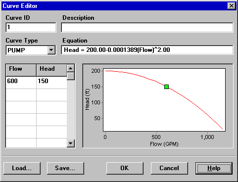
Curve Editor
The Curve Editor is a dialog form as shown in Fig. 6.1. To use the
Curve Editor, enter values for the following items (Table 6.8):
ID label of the curve (maximum of 15 numerals or characters)
Description
Optional description of what the curve represents
Curve Type
Type of curve
X-Y Data
X-Y data points for the curve
As you move between cells in the X-Y data table (or press the Enter
key) the curve is redrawn in the preview window. For single- and
three-point pump curves, the equation generated for the curve will be
displayed in the Equation box. Click the OK button to accept the
curve or the Cancel button to cancel your entries. You can also
click the Load button to load in curve data that was previously
saved to file or click the Save button to save the current
curve’s data to a file.
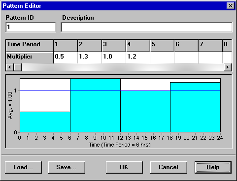
The Pattern Editor, displayed in Fig. 6.2, edits the properties of
a time pattern object. To use the Pattern Editor enter values for the
following items (Table 6.9):
ID label of the pattern (maximum
of 15 numerals or characters)
Description
Optional description of what the
pattern represents
Multipliers
Multiplier value for each time
period of the pattern.
As multipliers are entered, the preview chart is redrawn to provide a
visual depiction of the pattern. If you reach the end of the
available Time Periods when entering multipliers, simply hit the
Enter key to add on another period. When finished editing, click
the OK button to accept the pattern or the Cancel button to
cancel your entries. You can also click the Load button to load
in pattern data that was previously saved to file or click the
Save button to save the current pattern’s data to a file.
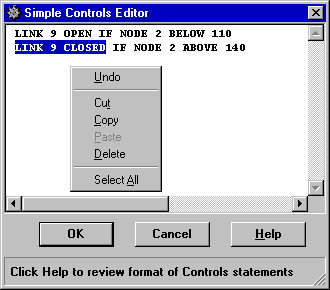
The Controls Editor, shown in Fig. 6.3, is a text editor window
used to edit both simple and rule-based controls. It has a standard
text-editing menu that is activated by right-clicking anywhere in the
Editor. The menu contains commands for Undo, Cut, Copy, Paste,
Delete, and Select All.
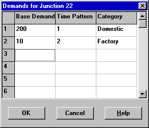
The Demand Editor is pictured in Fig. 6.4. It is used to assign
base demands and time patterns when there is more than one category
of water user at a junction. The editor is invoked from the Property
Editor by clicking the ellipsis button (or hitting the Enter key)
when the Demand Categories field has the focus.
The editor is a table containing three columns. Each category of
demand is entered as a new row in the table. The columns contain the
following information:
Base Demand: baseline or average demand for the category (required)
Time Pattern: ID label of time pattern used to allow demand to vary with time (optional)
Category: text label used to identify the demand category (optional)
The table initially is sized for 10 rows. If additional rows are
needed select any cell in the last row and hit the Enter key.
Note: By convention, the demand placed in the first row of the
editor will be considered the main category for the junction and will
appear in the Base Demand field of the Property Editor.
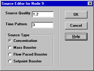
Source Quality Editor
The Source Quality Editor is a pop-up dialog used to describe the
quality of source flow entering the network at a specific node. This
source might represent the main treatment works, a well head or
satellite treatment facility, or an unwanted contaminant intrusion.
The dialog form, shown in Fig. 6.5, contains the following fields
(Table 6.10):
Baseline or average concentration
(or mass flow rate per minute) of
source – leave blank to remove
the source
Quality Pattern
ID label of time pattern used to
make source quality vary with
time – leave blank if not
applicable
A water quality source can be designated as a concentration or
booster source.
A concentration source fixes the concentration of any external
inflow entering the network, such as flow from a reservoir or from a
negative demand placed at a junction.
A mass booster source adds a fixed mass flow to that entering the
node from other points in the network.
A flow paced booster source adds a fixed concentration to that
resulting from the mixing of all inflow to the node from other points
in the network.
A setpoint booster source fixes the concentration of any flow
leaving the node (as long as the concentration resulting from all
inflow to the node is below the setpoint).
The concentration-type source is best used for nodes that represent
source water supplies or treatment works (e.g., reservoirs or nodes
assigned a negative demand). The booster-type source is best used to
model direct injection of a tracer or additional disinfectant into
the network or to model a contaminant intrusion.
The properties of an object displayed on the Network Map can be
copied and pasted into another object from the same category. To copy
the properties of an object to EPANET’s internal clipboard:
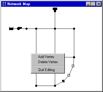
Links can be drawn as polylines containing any number of
straight-line segments that add change of direction and curvature to
the link. Once a link has been drawn on the map, interior points that
define these line segments can be added, deleted, and moved (see
Fig. 6.6). To edit the interior points of a link:
Select the link to edit on the Network Map and click on the
Map Toolbar (or select Edit >> Select Vertex from the Menu Bar,
or right-click on the link and select Vertices from the popup
menu).
The mouse pointer will change shape to an arrow tip, and any existing
vertex points on the link will be displayed with small handles around
them. To select a particular vertex, click the mouse over it.
To add a new vertex to the link, right-click the mouse and select
Add Vertex from the popup menu (or simply press the Insert
key on the keyboard).
To delete the currently selected vertex, right-click the mouse and
select Delete Vertex from the popup menu (or simply press the
Delete key on the keyboard).
To move a vertex to another location, drag it with the left mouse
button held down to its new position.
While in Vertex Selection mode you can begin editing the vertices for
another link by clicking on the link. To leave Vertex Selection mode,
right-click on the map and select Quit Editing from the popup
menu, or select any other button on the Map Toolbar.
A link can also have its direction reversed (i.e., its end nodes
switched) by right- clicking on it and selecting Reverse from the
pop-up menu that appears. This is useful for re-orienting pumps and
valves that originally were added in the wrong direction.
Select the object on the map or from the Data Browser.
Either:
Click on the Standard Toolbar
Click the same button on the Data Browser
Press the Delete key on the keyboard
Note: You can require that all deletions be confirmed before they
take effect. See the General Preferences page of the Program
Preferences dialog box described in Section 4.9.
To move a node or label to another location on the map:
Select the node or label.
With the left mouse button held down over the object, drag it to its
new location.
Release the left button.
Alternatively, new X and Y coordinates for the object can be typed in
manually in the Property Editor. Whenever a node is moved all links
connected to it are moved as well.
To select a group of objects that lie within an irregular region of
the network map:
Select Edit >> Select Region or click on the Map
Toolbar.
Draw a polygon fence line around the region of interest on the map
by clicking the left mouse button at each successive vertex of the
polygon.
Close the polygon by clicking the right button or by pressing the
Enter key; Cancel the selection by pressing the Escape key.
To select all objects currently in view on the map select Edit >>
Select All. (Objects outside the current viewing extent of the map
are not selected.)
Once a group of objects has been selected, you can edit a common
property (see the following section) or delete the selected objects
from the network. To do the latter, click or press the
Delete key.
Select the region of the map that will contain the group of objects
to be edited using the method described in previous section.
Select Edit >> Group Edit from the Menu Bar.
Define what to edit in the Group Edit dialog form that appears.
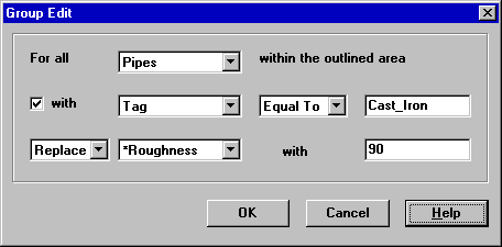
The Group Edit dialog form, shown in Fig. 6.7, is used to modify a
property for a selected group of objects. To use the dialog form:
Select a category of object (Junctions or Pipes) to edit.
Check the “with” box if you want to add a filter that will limit the
objects selected for editing. Select a property, relation and value
that define the filter. An example might be “with Diameter below 12”.
Select the type of change to make - Replace, Multiply, or Add To.
Select the property to change.
Enter the value that should replace, multiply, or be added to the
existing value.
, reservoir
, or tank
) to add from the Map Toolbar if it is not already depressed.
.
, pump
, or valve
) from the Map Toolbar if it is not already depressed.
on the Map Toolbar.
on the Map Toolbar or choose Select Object from the Edit menu.
on the Data Browser (or simply double-click the object on the map). The properties associated with each of these types of objects are described in Table 6.1 through Table 6.7.
on the Map Toolbar (or select Edit >> Select Vertex from the Menu Bar, or right-click on the link and select Vertices from the popup menu).
on the Standard Toolbar
on the Map Toolbar.