EPANET displays a map of the pipe network being modeled. This
chapter describes how you can manipulate this map to enhance your
visualization of the system being modeled.
One uses the Map Page of the Browser (Section 4.7) to select a node
and link parameter to view on the map. Parameters are viewed on the
map by using colors, as specified in the Map Legends (see below), to
display different ranges of values.
Node parameters available for viewing include:
Elevation
Base Demand (nominal or average demand)
Initial Quality (water quality at time zero)
*Actual Demand (total demand at current time)
*Hydraulic Head (elevation plus pressure head)
*Pressure
*Water Quality
Link parameters available for viewing include:
Length
Diameter
Roughness Coefficient
Bulk Reaction Coefficient
Wall Reaction Coefficient
*Flow Rate
*Velocity
*Headloss (per 1000 feet (or meters) of pipe)
*Friction Factor (as used in the Darcy-Weisbach headloss formula)
*Reaction Rate (average over length of pipe)
*Water Quality (average over length of pipe)
The items marked with asterisks are computed quantities whose values
will only be available if a successful analysis has been run on the
network (see Chapter Analyzing a Network).
The physical dimensions of the map must be defined so that map
coordinates can be properly scaled to the computer’s video display.
To set the map’s dimensions:
Select View >> Dimensions.
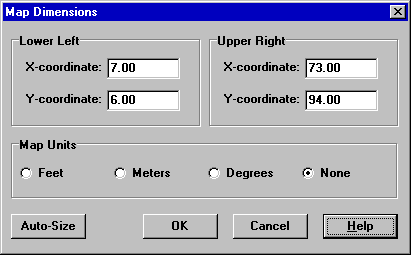
Enter new dimension information into the Map Dimensions dialog that
appears (see Fig. 7.1) or click the Auto-Size button to have
EPANET compute dimensions based on the coordinates of objects
currently included in the network.
The X and Y coordinates of the
lower left point on the map.
Upper Right Coordinates
The X and Y coordinates of the
upper right point on the map.
Map Units
Units used to measure distances
on the map. Choices are Feet,
Meters, Degrees, and None (i.e.,
arbitrary units).
Note: If you are going to use a backdrop map with automatic pipe
length calculation, then it is recommended that you set the map
dimensions immediately after creating a new project. Map distance
units can be different from pipe length units. The latter (feet or
meters) depend on whether flow rates are expressed in US or metric
units. EPANET will automatically convert units if necessary.
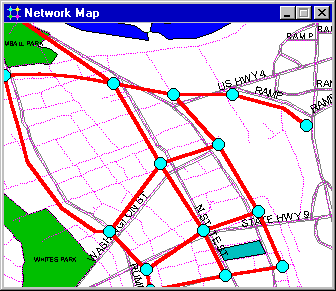
EPANET can display a backdrop map behind the pipe network map. The
backdrop map might be a street map, utility map, topographic map,
site development plan, or any other picture or drawing that might be
useful. For example, using a street map would simplify the process of
adding pipes to the network since one could essentially digitize the
network’s nodes and links directly on top of it (Fig. 7.2).
The backdrop map must be a Windows enhanced metafile or bitmap
created outside of EPANET. Once imported, its features cannot be
edited, although its scale and extent will change as the map window
is zoomed and panned. For this reason metafiles work better than
bitmaps since they will not loose resolution when re-scaled. Most
CAD and GIS programs have the ability to save their drawings and maps
as metafiles.
Selecting View >> Backdrop from the Menu Bar will display a
sub-menu with the following commands:
Load (loads a backdrop map file into the project)
Unload (unloads the backdrop map from the project)
Align (aligns the pipe network with the backdrop)
Show/Hide (toggles the display of the backdrop on and off)
When first loaded, the backdrop image is placed with its upper left
corner coinciding with that of the network’s bounding rectangle. The
backdrop can be re-positioned relative to the network map by
selecting View >> Backdrop >> Align. This allows an outline of
the pipe network to be moved across the backdrop (by moving the mouse
with the left button held down) until one decides that it lines up
properly with the backdrop. The name of the backdrop file and its
current alignment are saved along with the rest of a project’s data
whenever the project is saved to file.
For best results in using a backdrop map:
Use a metafile, not a bitmap.
Dimension the network map so that its bounding rectangle has the same
aspect ratio (width-to-height ratio) as the backdrop.
Select View >> Zoom In or click on the Map Toolbar.
To zoom in 100%, move the mouse to the center of the zoom area and
click the left button.
To perform a custom zoom, move the mouse to the upper left corner of
the zoom area and with the left button pressed down, draw a
rectangular outline around the zoom area. Then release the left
button.
To Zoom Out on the map:
Select View >> Zoom Out or click on the Map Toolbar.
Move the mouse to the center of the new zoom area and click the left
button.
The map will be returned to its previous zoom level.
To find a node or link on the map whose ID label is known:
Select View >> Find or click on the Standard
Toolbar.
In the Map Finder dialog box that appears, select Node or
Link and enter an ID label.
Click Find.
If the node/link exists it will be highlighted on the map and in the
Browser. If the map is currently zoomed in and the node/link falls
outside the current map boundaries, the map will be panned so that
the node/link comes into view. The Map Finder dialog will also list
the ID labels of the links that connect to a found node or the nodes
attached to a found link.
To find a listing of all nodes that serve as water quality sources:
Select View >> Find or click on the Standard
Toolbar.
In the Map Finder dialog box that appears, select Sources.
Click Find.
The ID labels of all water quality source nodes will be listed in the
Map Finder. Clicking on any ID label will highlight that node on the
map.
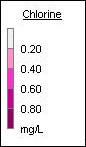
There are three types of map legends that can be
displayed. The Node and Link Legends associate a color with a range
of values for the current parameter being viewed on the map (see Fig. 7.3).
The Time Legend displays the clock time of the simulation time period being viewed. To display or hide any of these legends check or uncheck the
legend from the View >> Legends menu or right- click over the map
and do the same from the popup menu that appears. Double-clicking the
mouse over it can also hide a visible legend.
To move a legend to another location:
Press the left mouse button over the legend.
With the button held down, drag the legend to its new location and release the button.
To edit the Node Legend:
Either select View >> Legends >> Modify >> Node or right-click on the legend if it is visible.
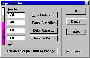
Use the Legend Editor dialog form that appears (see Fig. 7.4) to modify the legend’s colors and intervals.
A similar method is used to edit the Link Legend.
The Legend Editor (Fig. 7.4) is used to set numerical ranges to
which different colors are assigned for viewing a particular
parameter on the network map. It works as follows:
Numerical values, in increasing order, are entered in the edit boxes to define the ranges. Not all four boxes need to have values.
To change a color, click on its color band in the Editor and then select a new color from the Color Dialog box that will appear.
Click the Equal Intervals button to assign ranges based on dividing the range of the parameter at the current time period into equal intervals.
Click the Equal Quantiles button to assign ranges so that there are equal numbers of objects within each range, based on values that exist at the current time period.
The Color Ramp button is used to select from a list of built-in color schemes.
The Reverse Colors button reverses the ordering of the current set of colors (the color in the lowest range becomes that of the highest range and so on).
Check Framed if you want a frame drawn around the legend.
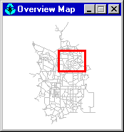
The Overview Map allows you to see where in terms of the overall
system the main network map is currently focused. This zoom area is
depicted by the rectangular boundary displayed on the Overview Map (Fig. 7.5).
As you drag this rectangle to another position the view within the
main map will follow suit. The Overview Map can be toggled on and off
by selecting View >> Overview Map. Clicking the mouse on its
title bar will update its map image to match that of the main network
map.
Displays map labels (labels will
be hidden unless this option is
checked)
Use Transparent Text
Displays label with a transparent
background (otherwise an opaque
background is used)
At Zoom Of
Selects minimum zoom at which
labels should be displayed;
labels will be hidden at zooms
smaller than this unless they are
meter labels
Notation Options
The Notation page of the Map Options dialog form determines what kind
of annotation is provided alongside of the nodes and links of the
map (Table 7.5).
Displays value of current node
parameter being viewed
Display Link IDs
Displays link ID labels
Display Link Values
Displays values of current link
parameter being viewed
Use Transparent Text
Displays text with a transparent
background (otherwise an opaque
background is used)
At Zoom Of
Selects minimum zoom at which
notation should be displayed; all
notation will be hidden at zooms
smaller than this
Note: Values of the current viewing parameter at only specific
nodes and links can be displayed by creating Map Labels with meters
for those objects. See Section 6.2 and Section 6.4 as well as Table 6.7.
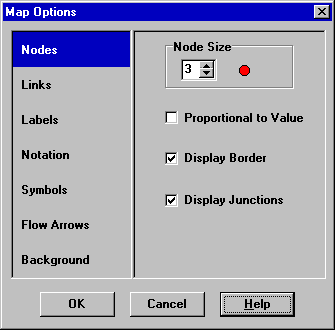
Symbol Options
The Symbols page of the Map Options dialog determines which types of
objects are represented with special symbols on the map (Table 7.6).
on the Map Toolbar.
on the Map Toolbar.
on the Map Toolbar.
on the Standard Toolbar.
on the Standard Toolbar when the Map window has the focus