%matplotlib inline
# tag: remove-cell applied

Continuous Data with Bayesian Model Averaging¶

Table of Contents¶

Single model fit - LOUD
Multiple model fit (sessions) - LOUD
Running expanded suite analyses

Bayesian model averaging is currently available for continuous datasets in pybmdsusing the Bayesian LOUD (Leveraging Optimized Unified prior Distributions) method. Here, we describe how to run a continuous analysis using a single model, or model averaging using the standard BMDS suite of models or the expanded suite using PROAST or EFSA models. Additionally, we demonstrate how to plot your results.

Single model fit - LOUD¶

You can run individual models using the Bayesian LOUD approach rather than running all models and finding the model average.

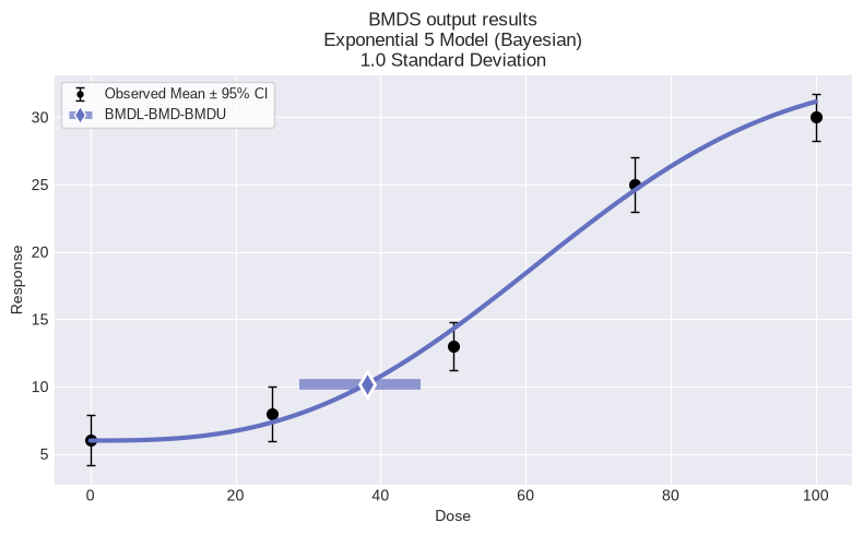
To run the Exponential 5 model:

import pybmds
from pybmds.models import continuous

# create a continuous dataset
dataset = pybmds.ContinuousDataset(
    doses=[0, 25, 50, 75, 100],
    ns=[20, 20, 20, 20, 20],
    means=[6, 8, 13, 25, 30],
    stdevs=[4, 4.3, 3.8, 4.4, 3.7],
)

# Single model fit using LOUD model averaging 
model = continuous.ExponentialM5(
    dataset=dataset,
    settings={
        "priors": pybmds.PriorClass.bayesian_loud,
        "seed": 123,
    },
)

model.execute()

print(model.text())
fig = model.plot()

     Exponential 5 Model      
══════════════════════════════

Version: pybmds 26.1 (bmdscore 26.1)

Input Summary:
╒══════════════════════════════╤════════════════════════════╕
│ BMR                          │ 1.0 Standard Deviation     │
│ Distribution                 │ Normal + Constant variance │
│ Modeling Direction           │ Up (↑)                     │
│ Confidence Level (one sided) │ 0.95                       │
│ Modeling Approach            │ Bayesian                   │
╘══════════════════════════════╧════════════════════════════╛

Parameter Settings:
╒═════════════╤════════════════╤════════════════════════════════════════════════════════════╕
│ Parameter   │ Distribution   │ Definition                                                 │
╞═════════════╪════════════════╪════════════════════════════════════════════════════════════╡
│ m0          │ Student_t      │ df=19.0, loc=6.0, scale=0.917662935482247                  │
│ m1          │ Student_t      │ df=19.0, loc=30.0, scale=0.8488382153210785                │
│ b           │ Lognormal      │ initial=0.0, stdev=2.0, min=0.0, max=18.0                  │
│ d           │ Lognormal      │ initial=0.47, stdev=0.421, min=0.0, max=18.0               │
│ Var         │ Gamma          │ shape=19.5, scale=296.90000000000003, min=0.0, max=10000.0 │
╘═════════════╧════════════════╧════════════════════════════════════════════════════════════╛

Modeling Summary:
╒════════════════╤══════════╕
│ BMD            │   38.09  │
│ BMDL           │   28.816 │
│ BMDU           │   45.52  │
│ Log-Likelihood │ -170.976 │
│ P-Value        │    0.648 │
│ WAIC           │ -175.458 │
╘════════════════╧══════════╛

Model Parameters:
╒════════════╤════════════╤════════════╤══════════════╕
│ Variable   │   Estimate │ On Bound   │    Std Error │
╞════════════╪════════════╪════════════╪══════════════╡
│ a          │  5.99176   │ no         │   0.870433   │
│ b          │  0.0140084 │ no         │   0.00338004 │
│ c          │  5.53551   │ no         │ 959.768      │
│ d          │  2.84008   │ no         │   0.732578   │
│ alpha      │ 17.1304    │ no         │   2.62651    │
╘════════════╧════════════╧════════════╧══════════════╛

Goodness of Fit:
╒════════╤═════╤═══════════════╤═════════════════════╤═══════════════════╕
│   Dose │   N │   Sample Mean │   Model Fitted Mean │   Scaled Residual │
╞════════╪═════╪═══════════════╪═════════════════════╪═══════════════════╡
│      0 │  20 │             6 │             6.06661 │        -0.0720744 │
│     25 │  20 │             8 │             7.43446 │         0.611935  │
│     50 │  20 │            13 │            14.2716  │        -1.37589   │
│     75 │  20 │            25 │            24.3542  │         0.698822  │
│    100 │  20 │            30 │            31       │        -1.08199   │
╘════════╧═════╧═══════════════╧═════════════════════╧═══════════════════╛
╒════════╤═════╤═════════════╤═══════════════════╕
│   Dose │   N │   Sample SD │   Model Fitted SD │
╞════════╪═════╪═════════════╪═══════════════════╡
│      0 │  20 │         4   │           4.13305 │
│     25 │  20 │         4.3 │           4.13305 │
│     50 │  20 │         3.8 │           4.13305 │
│     75 │  20 │         4.4 │           4.13305 │
│    100 │  20 │         3.7 │           4.13305 │
╘════════╧═════╧═════════════╧═══════════════════╛

../_images/21a7688fdc6708f37eae51aecbb3fb576a0b9c7f911d793b866a6aa321cc7734.png

Multiple model fit (sessions) - LOUD¶

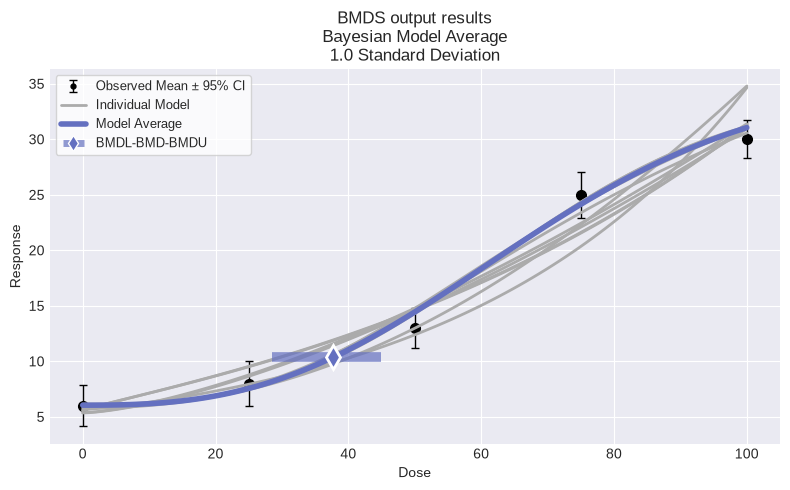
To run LOUD Bayesian model averaging for continuous data using the standard BMDS suite of models, chainging the default MCMC settings to chains = 4, iterations/chain = 12,500, and burn-in/chain = 1,250:

import pybmds

# create a continuous dataset
dataset = pybmds.ContinuousDataset(
    doses=[0, 25, 50, 75, 100],
    ns=[20, 20, 20, 20, 20],
    means=[6, 8, 13, 25, 30],
    stdevs=[4, 4.3, 3.8, 4.4, 3.7],
)

# LOUD model averaging using the standard BMDS continuous suite
session1 = pybmds.Session(dataset=dataset)

settings = {
    "n_chains": 4,
    "samples": 7500,
    "burnin": 1500,
    "seed": 123,
}

session1.add_default_bayesian_models(
    settings=settings,
    prior_class=pybmds.PriorClass.bayesian_loud,
    model_average=True,      # add model averaging
    include_extended=False,  # standard suite only (not PROAST/EFSA-expanded)
)
session1.execute()

# summarize model-averaged result
res1 = session1.model_average.results
print(f"BMD = {res1.bmd:.2f} [{res1.bmdl:.2f}, {res1.bmdu:.2f}]")

# optional: plot model fits and model-average curve
fig1 = session1.plot(colorize=False)

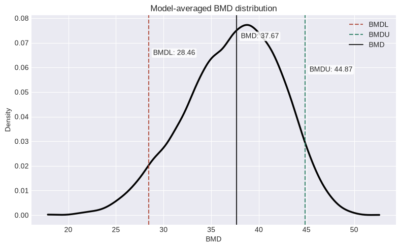
BMD = 37.67 [28.46, 44.87]

../_images/b79ececca721ad210ac074c516081c7457648993e3ad825836a842e30b70cd56.png

confirm the MCMC settings:

model = session1.models[0]  # or whichever model you want to inspect
print("samples:", model.settings.samples)
print("burnin:", model.settings.burnin)
print("n_chains:", model.settings.n_chains)
print("seed:", model.settings.seed)

samples: 7500
burnin: 1500
n_chains: 4
seed: 123

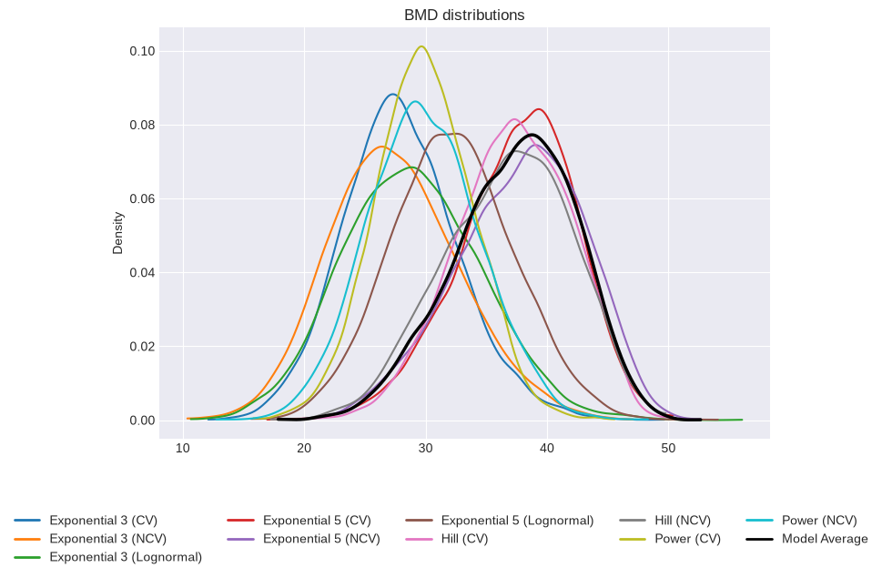
To print the model average distribution plot and BMD distribution overlay plot:

from pybmds.plotting.LOUD import get_model_average_figures
from IPython.display import display

figs1 = get_model_average_figures(session1, compressed=True)

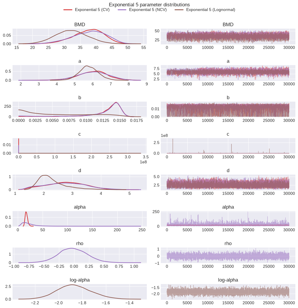
../_images/35673285791679870fd0e2ddac629d644bd92a5c9ee160331c028b7f2fbf40c1.png

../_images/599fe2055cb1e7fd71208e0870a1de1c388e0597a6c06f6b6efe32014d8afc3a.png

To print the trace plots for an individual model:

target_model = "Exponential 5 (CV)"

for group in figs1["parameter_groups"]:
    if target_model in group["model_names"]:
        print("Trace plot for:", target_model)
        display(group["trace_figure"])
        break

Trace plot for: Exponential 5 (CV)

../_images/b831c581f3ed63c94e1559312fd4262b37647d73f8548f868b787d78d3f588b6.png

To print out the MCMC summary table for model-specific BMDs:

display(figs1["bmd_summary"])

	Posterior Weights	BMD	Median Absolute Deviation	R-hat	Markov Chain Standard Error (Median)	Bulk Effective Sample Size	Tail Effective Sample Size	BMDL	BMDU
model
Exponential 3 (CV)	0.0001	27.713742	3.130151	1.000553	0.077314	3532.539389	3635.102721	20.524218	36.144611
Exponential 3 (NCV)	0.00013	27.202288	3.598425	1.000653	0.091618	3348.843862	5021.118557	19.070434	36.698632
Exponential 3 (Lognormal)	0.000231	28.753017	3.874337	1.001270	0.081926	4395.546505	5298.778052	19.909502	38.464278
Exponential 5 (CV)	0.433926	37.924254	3.231709	1.006425	0.126517	1542.898873	2242.326970	28.936044	44.696075
Exponential 5 (NCV)	0.222101	38.134441	3.654316	1.004580	0.158786	1172.210400	1520.564045	28.307410	45.694360
Exponential 5 (Lognormal)	0.004513	32.110365	3.387915	1.000798	0.105221	2488.299744	2788.053360	24.106922	40.752724
Hill (CV)	0.220992	37.366367	3.324890	1.009036	0.163752	933.793578	1076.216157	29.125036	44.623698
Hill (NCV)	0.106372	37.100968	3.691206	1.023774	0.302109	307.355793	940.821396	27.619137	44.755811
Power (CV)	0.005524	29.812821	2.672861	1.001856	0.064351	3658.890175	5200.650325	23.409474	36.521412
Power (NCV)	0.006111	29.700620	3.126839	1.001070	0.085998	3361.000700	5120.143799	22.484969	37.650516
MA_BMD	None	37.669465	3.456039	1.002709	0.084358	4066.483673	5449.214040	28.460390	44.869556

To display a summary table of results without MCMC output:

from IPython.display import display

bayes_summary1 = (
session1.to_df(clean=False)
[[
"model_name",
"model_prior",
"model_posterior",
"bmdl",
"bmd",
"bmdu",
"residual_at_lowest_dose",
"residual_of_interest",
]]
.rename(columns={
"model_name": "Model",
"model_prior": "Prior Weights",
"model_posterior": "Posterior Weights",
"bmdl": "BMDL",
"bmd": "BMD",
"bmdu": "BMDU",
"residual_at_lowest_dose": "Residual at Control",
"residual_of_interest": "Scaled Residual",
})
)

df1 = bayes_summary1
display(df1)

	Model	Prior Weights	Posterior Weights	BMDL	BMD	BMDU	Residual at Control	Scaled Residual
0	Power (CV)	0.1	0.005524	23.409474	29.812821	36.521412	0.654874	-0.730541
1	Power (NCV)	0.1	0.006111	22.484969	29.700620	37.650516	0.647174	-0.717251
2	Hill (CV)	0.1	0.220992	29.125036	37.366367	44.623698	-0.005627	0.592655
3	Hill (NCV)	0.1	0.106372	27.619137	37.100968	44.755811	0.034109	0.427376
4	Exponential 3 (CV)	0.1	0.000100	20.524218	27.713742	36.144611	0.488212	-1.507548
5	Exponential 3 (NCV)	0.1	0.000130	19.070434	27.202288	36.698632	0.489941	-1.477439
6	Exponential 3 (Lognormal)	0.1	0.000231	19.909502	28.753017	38.464278	-0.257044	-0.792491
7	Exponential 5 (CV)	0.1	0.433926	28.936044	37.924254	44.696075	-0.044534	-1.371802
8	Exponential 5 (NCV)	0.1	0.222101	28.307410	38.134441	45.694360	-0.028423	-1.510050
9	Exponential 5 (Lognormal)	0.1	0.004513	24.106922	32.110365	40.752724	-0.390961	0.281088
10	Model average	NaN	NaN	28.460390	37.669465	44.869556	NaN	NaN

Running Expanded Suite analyses¶

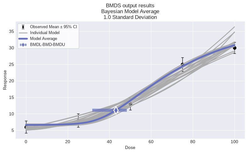
To run LOUD Bayesian model averaging for continuous data using the expanded suite of models (i.e., BMDS + PROAST + EFSA models) and the same changes to the MCMC settings:

# LOUD model averaging using the expanded BMDS/PROAST/EFSA continuous suite
session2 = pybmds.Session(dataset=dataset)

settings = {
    "n_chains": 4,
    "samples": 12500,
    "burnin": 1250,
    "seed": 123,
}

session2.add_default_bayesian_models(
    settings=settings,
    prior_class=pybmds.PriorClass.bayesian_loud,
    model_average=True,      # add model averaging
    include_extended=True,  # expanded BMDS/PROAST/EFSA suite  
)
session2.execute()

# summarize model-averaged result
res2 = session2.model_average.results
print(f"BMD = {res2.bmd:.2f} [{res2.bmdl:.2f}, {res2.bmdu:.2f}]")

# optional: plot model fits and model-average curve
fig2 = session2.plot(colorize=False)

BMD = 43.04 [31.79, 48.31]

../_images/325a61c4706f4e2072648ce8650ec53634a4e02eeb27d1db5cbadb3b4ea4614e.png

And to print out a summary table:

bayes_summary2 = (
session2.to_df(clean=False)
[[
"model_name",
"model_prior",
"model_posterior",
"bmdl",
"bmd",
"bmdu",
"residual_at_lowest_dose",
"residual_of_interest",
]]
.rename(columns={
"model_name": "Model",
"model_prior": "Prior Weights",
"model_posterior": "Posterior Weights",
"bmdl": "BMDL",
"bmd": "BMD",
"bmdu": "BMDU",
"residual_at_lowest_dose": "Residual at Control",
"residual_of_interest": "Scaled Residual",
})
)

df2 = bayes_summary2
display(df2)

	Model	Prior Weights	Posterior Weights	BMDL	BMD	BMDU	Residual at Control	Scaled Residual
0	Power (CV)	0.043478	0.000684	23.320379	30.020833	37.222190	0.621267	-0.723924
1	Power (NCV)	0.043478	0.000803	22.433512	29.743756	37.515730	0.638285	-0.735962
2	Exponential 3 (CV)	0.043478	0.000019	20.735498	27.884262	36.077092	0.480743	-1.473752
3	Exponential 3 (NCV)	0.043478	0.000026	19.272916	27.462354	36.759717	0.507562	-1.441722
4	Exponential 3 (Lognormal)	0.043478	0.000040	20.022366	28.709927	38.495125	-0.269027	-0.801789
5	Exponential 5 (CV)	0.043478	0.081558	29.357445	38.251143	45.031112	-0.084482	-1.333394
6	Exponential 5 (NCV)	0.043478	0.036282	28.495324	38.153960	45.882031	-0.033337	-1.474722
7	Exponential 5 (Lognormal)	0.043478	0.000751	24.205000	32.111892	41.052494	-0.401873	0.247314
8	Multiplicative Hill (CV)	0.043478	0.019055	27.363897	35.591912	44.284809	0.340373	0.508337
9	Multiplicative Hill (NCV)	0.043478	0.024259	28.091041	37.387241	44.824842	0.006530	0.501154
10	Multiplicative Hill (Lognormal)	0.043478	0.000707	23.243059	31.032290	39.491500	-0.416909	0.215891
11	Inverse Exponential (CV)	0.043478	0.326772	38.549579	44.454044	48.718841	-0.965812	-0.533044
12	Inverse Exponential (NCV)	0.043478	0.225904	38.211465	44.557795	48.947162	-0.904495	-0.543087
13	Inverse Exponential (Lognormal)	0.043478	0.001339	31.947999	40.376899	46.395964	-1.497278	-0.868936
14	Lognormal (CV)	0.043478	0.148303	34.484437	42.224672	47.792697	-0.681032	-0.865360
15	Lognormal (NCV)	0.043478	0.100286	34.104053	42.237935	47.900101	-0.586153	-0.873658
16	Lognormal (Lognormal)	0.043478	0.001510	28.549439	36.668372	44.300996	-1.079545	0.880736
17	Continuous Gamma (CV)	0.043478	0.003493	25.924380	32.729557	39.063945	0.445551	-0.179953
18	Continuous Gamma (NCV)	0.043478	0.003476	25.256053	32.981824	40.216759	0.426504	-0.150920
19	Continuous Gamma (Lognormal)	0.043478	0.000716	22.732790	30.159293	38.161934	-0.347496	0.127304
20	LMS 2-Stage (CV)	0.043478	0.012542	25.833048	30.009946	33.971359	0.977008	-0.051682
21	LMS 2-Stage (NCV)	0.043478	0.011380	25.199782	30.161451	35.378247	0.944964	-0.071205
22	LMS 2-Stage (Lognormal)	0.043478	0.000094	18.996862	23.633158	28.605497	0.509954	-0.613211
23	Model average	NaN	NaN	31.794766	43.035840	48.313120	NaN	NaN

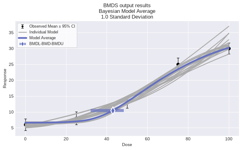
To run LOUD Bayesian model averaging for continuous data using the just the PROAST and EFSA models:

# dataset
dataset = pybmds.ContinuousDataset(
    doses=[0, 25, 50, 75, 100],
    ns=[20, 20, 20, 20, 20],
    means=[6, 8, 13, 25, 30],
    stdevs=[4, 4.3, 3.8, 4.4, 3.7],
)

session3 = pybmds.Session(dataset=dataset)

# Expanded models only (PROAST/EFSA-style set), LOUD priors
expanded_models = [
    pybmds.Models.ExponentialM3,
    pybmds.Models.ExponentialM5,
    pybmds.Models.MultiplicativeHill,
    pybmds.Models.InverseExponential,
    pybmds.Models.Lognormal,
    pybmds.Models.ContinuousGamma,
    pybmds.Models.LMS2,
]

# add all three disttypes (example: constant variance)
dist_types = [
    pybmds.ContinuousDistType.normal,
    pybmds.ContinuousDistType.normal_ncv,
    pybmds.ContinuousDistType.log_normal,
]

for model_name in expanded_models:
    for dt in dist_types:
        session3.add_model(
            model_name,
            settings={
                "n_chains": 4,
                "samples": 12500,
                "burnin": 1250,
                "seed": 123,
                "priors": pybmds.PriorClass.bayesian_loud,
                "disttype": dt,
            },
        )

session3.add_model_averaging()
session3.execute()

res3 = session3.model_average.results
print(f"BMD = {res3.bmd:.2f} [{res3.bmdl:.2f}, {res3.bmdu:.2f}]")
fig3 = session3.plot(colorize=False)

BMD = 43.03 [32.11, 48.44]

../_images/68593f75f69f680d00f037812f5ab0699638d629805c1064d3dd797e82bb2fff.png

To print a summary table for the EFSA and PROAST models:

bayes_summary3 = (
session3.to_df(clean=False)
[[
"model_name",
"model_prior",
"model_posterior",
"bmdl",
"bmd",
"bmdu",
"residual_at_lowest_dose",
"residual_of_interest",
]]
.rename(columns={
"model_name": "Model",
"model_prior": "Prior Weights",
"model_posterior": "Posterior Weights",
"bmdl": "BMDL",
"bmd": "BMD",
"bmdu": "BMDU",
"residual_at_lowest_dose": "Residual at Control",
"residual_of_interest": "Scaled Residual",
})
)

df3 = bayes_summary3
display(df3)

	Model	Prior Weights	Posterior Weights	BMDL	BMD	BMDU	Residual at Control	Scaled Residual
0	Exponential 3 (CV)	0.047619	0.000020	20.735498	27.884262	36.077092	0.480743	-1.473752
1	Exponential 3 (NCV)	0.047619	0.000027	19.272916	27.462354	36.759717	0.507562	-1.441722
2	Exponential 3 (Lognormal)	0.047619	0.000041	20.022366	28.709927	38.495125	-0.269027	-0.801789
3	Exponential 5 (CV)	0.047619	0.084702	29.357445	38.251143	45.031112	-0.084482	-1.333394
4	Exponential 5 (NCV)	0.047619	0.037681	28.495324	38.153960	45.882031	-0.033337	-1.474722
5	Exponential 5 (Lognormal)	0.047619	0.000780	24.205000	32.111892	41.052494	-0.401873	0.247314
6	Multiplicative Hill (CV)	0.047619	0.032674	29.004702	36.544912	44.427208	0.115889	0.602831
7	Multiplicative Hill (NCV)	0.047619	0.012750	27.035375	36.588446	44.145742	0.112514	0.459696
8	Multiplicative Hill (Lognormal)	0.047619	0.000755	23.301830	31.206884	39.892231	-0.443085	0.225538
9	Inverse Exponential (CV)	0.047619	0.328863	38.289200	44.476537	48.759161	-0.967364	-0.541460
10	Inverse Exponential (NCV)	0.047619	0.224466	38.166546	44.676218	49.162159	-0.933116	-0.541448
11	Inverse Exponential (Lognormal)	0.047619	0.001376	32.185155	40.506164	46.460730	-1.511233	-0.804672
12	Lognormal (CV)	0.047619	0.122408	34.188231	41.798920	47.580865	-0.617095	-1.015857
13	Lognormal (NCV)	0.047619	0.123486	34.290002	42.409682	48.142654	-0.636936	-0.913325
14	Lognormal (Lognormal)	0.047619	0.001556	28.676872	36.627345	44.309198	-1.086399	0.871247
15	Continuous Gamma (CV)	0.047619	0.003642	26.166524	32.481383	39.494109	0.511815	-0.142416
16	Continuous Gamma (NCV)	0.047619	0.003232	25.201830	32.553437	39.584163	0.455265	-0.238364
17	Continuous Gamma (Lognormal)	0.047619	0.000708	22.755627	30.163644	38.176235	-0.334919	0.131343
18	LMS 2-Stage (CV)	0.047619	0.010754	25.752656	30.016642	34.091165	0.961947	-0.069768
19	LMS 2-Stage (NCV)	0.047619	0.009976	25.094588	30.095447	35.416868	0.952147	-0.075418
20	LMS 2-Stage (Lognormal)	0.047619	0.000104	19.017107	23.629628	28.656197	0.503095	-0.613528
21	Model average	NaN	NaN	32.108627	43.028231	48.441178	NaN	NaN

To compare the model averaged results for all three analyses using different model suites:

import pandas as pd

def ma_point_summary(session, label):
    if session.model_average is None:
        raise ValueError(f"{label} has no model average.")
    r = session.model_average.results
    return {
        "Session": label,
        "BMDL": float(r.bmdl),
        "BMD": float(r.bmd),
        "BMDU": float(r.bmdu),
    }

comparison = pd.DataFrame([
    ma_point_summary(session1, "Session 1 (BMDS only)"),
    ma_point_summary(session2, "Session 2 (BMDS + Expanded)"),
    ma_point_summary(session3, "Session 3 (Expanded only)"),
])

comparison

	Session	BMDL	BMD	BMDU
0	Session 1 (BMDS only)	28.460390	37.669465	44.869556
1	Session 2 (BMDS + Expanded)	31.794766	43.035840	48.313120
2	Session 3 (Expanded only)	32.108627	43.028231	48.441178