Dichotomous Endpoints
BMDS includes models for dichotomous endpoints in which the observations are independent of each other. In these models, the dose-response model defines the probability that an experimental unit (e.g., a rat or a mouse in a standard, non-nested toxicological study) will have an adverse response at a given dose. The actual number of animals that have an adverse response is assumed to be binomially distributed.
A specific example of such a dataset is a study in which adult animals are exposed to different concentrations of a toxicant and then evaluated for the presence of liver toxicity manifested as increased histopathological lesions.
For models for dichotomous endpoints in which the responses are nested (for example, pups within litters, and litters nested within doses), see Nested Dichotomous Endpoints.
For dichotomous cancer models, and the combination of model predictions for multiple tumor endpoints, see Multiple Tumor Analysis.
For more information on the Bayesian implementation of the dichotomous models, see Bayesian Dichotomous Analysis.
Dichotomous Response Models
BMDS offers the traditional MLE dichotomous response models available in previous versions of BMDS plus Bayesian versions of each model, and a Bayesian model averaging feature.
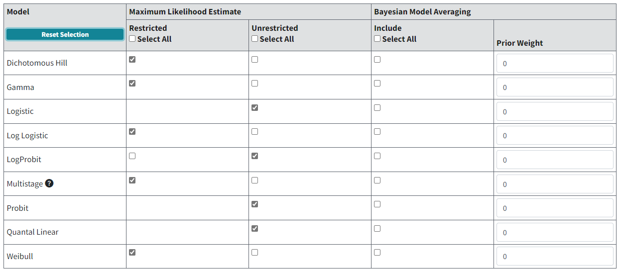
Figure 76. Default dichotomous model selection.
Most MLE models can be run restricted or unrestricted. The EPA default recommendation for initial runs is to restrict the Dichotomous Hill, Gamma, Log-Logistic, Multistage, and Weibull models and un-restrict the Logistic, Log-Probit, Probit and Quantal Linear models. Note that the Logistic, Probit, and Quantal Linear models have no restricted option (U.S. EPA, 2012).
See Individual Dichotomous Models and their Respective Parameters for the effect of the user selecting the restricted version of the models (refer to the paragraphs in the Notes fields). In general, the restrictions prevent the slope of the dose-response curve from becoming infinite at 0 dose. This is often considered to be biologically unrealistic and can lead to numerical problems when computing confidence limits, so several authors have recommended restricting the appropriate parameter.
A BMDS Online analysis can have a maximum of six datasets for dichotomous endpoints.
Maximum Multistage Degree
The dataset-specific Maximum multistage degree picklist will contain choices for degree 1 to the lesser of \(N‑1\) or 4.
The default value for number degrees to run will be the lesser of \(N‑1\) or 3, but the user can change this to a higher number of degrees up to the lesser of \(N‑1\) or 4.
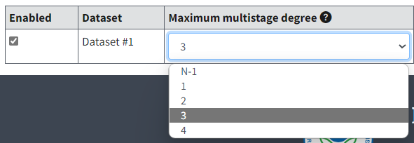
Figure 77. Maximum Multistage Degrees for dichotomous datasets.
Hovering over the help text icon for Maximum multistage degree displays the following text:
Note
Studies have indicated that higher degree polynomial models are not warranted in that they generally do not sufficiently improve fit over simpler models (Nitcheva et al., 2007; PMC2040324). Complex models also increase computer processing time and the chance of model failure.
Option Sets
On the Settings tab, the user can define up to six Option Sets in BMDS Online (unlimited in BMDS Desktop and pybmds) to apply to multiple user-selected models and multiple user-selected datasets in a single batch process.
Select the blue Plus button in the table header to define a new Option Set configuration row; select the red Trash Can button to delete the row.
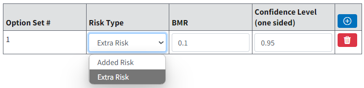
Figure 78. Dichotomous Model options
Risk Type
Choices for the Risk Type option are Extra Risk (Default) or Added Risk.
Added risk is the additional proportion of the total experimental units that respond in the presence of the dose, or the predicted probability of response at dose \(d\), \(P(d)\), minus the predicted probability of response in the absence of exposure, \(P(0)\):
Extra risk is the additional risk divided by the predicted proportion of animals that will not respond in the absence of exposure (\(1\ - \ P(0))\):
BMR
The BMR is the value of risk (extra or added, as specified by the user) for which a BMD is estimated. BMR must be between 0 and 1 (not inclusive).
If \(P(0)\ > \ 0\), then values for the BMR greater than \(1 - \ P(0)\) will result in an error when the risk type is added risk. That is because the maximum added risk that can ever be achieved is \(1 - \ P(0)\). In practice, this should not typically be an issue because one usually is interested in BMR values in the range of 0.01 to around 0.10.
BMR and Plots
The response associated with the BMR that is displayed in the graphical model output will only be the same as the BMR when \(P(0)\ = \ 0\).
This is because to obtain the actual response value one must solve for \(P(d)\) in the equation for added or extra risk discussed above.
The horizontal bar depicting the response level used to derive the BMD (Figure 79.) that is displayed in the graphical model output will only be the same as the user-defined BMR (e.g., 10% Extra Risk) when the response at background, P(0), equals zero.
When P(0) does not equal zero, the true response level can be calculated using the Extra Risk equation described in Risk Type
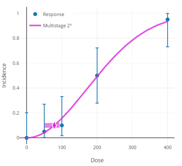
Figure 79. Results plot, with horizontal bar centered on the y-axis at the modeled BMR.
Confidence Level (one sided)
The Confidence Level is a fraction between 0 and 1; 0.95 is recommended by EPA (U.S. EPA, 2012).
The value for confidence level must be between 0 and 1 (not inclusive). For a confidence level of \(x\), BMDS will output BMDL and BMDU estimates, each of which is a one-sided confidence bound at level \(x\).
For example, if the user sets the confidence level to 0.95 (the default), then the BMDL is a 95% one-sided lower confidence bound for the BMD estimate; the BMDU is a 95% one-sided lower upper confidence bound for the BMD estimate. In that example, the range from BMDL to BMDU would constitute a 90% confidence interval (5% in each tail outside that interval).
Specific Dichotomous Results
Goodness of Fit Table
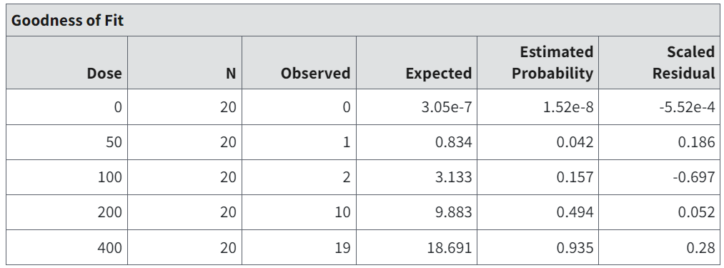
Figure 80. Goodness of Fit table for MLE Dichotomous.
The Goodness of Fit table in the individual model results shows a listing of the data (N and Observed), the model-estimated probability of response (Estimated Probability), and corresponding expected number of responders (Expected). This is a good place for the user to assess the appropriateness of the model, in addition to the overall goodness-of-fit statistics reported in the Summary table (refer to Summary Table of Key Fit Statistics (All Endpoints) and Analysis of Deviance Table). If a model fits well, the observed and expected number of responders should be relatively close.
The scaled residual values printed at the end of the table are defined as follows:
where Expected is the predicted number of responders from the model and SE equals the estimated standard error of that predicted number. For these models, the estimated standard error is equal to \(\sqrt{\lbrack n \times p \times (1 - p)\rbrack}\), where
\(n\) is the sample size (\(N\) in the goodness-of-fit table), and
\(p\) is the model-predicted probability of response (Estimated Probability in the goodness-of-fit table).
The fit of the model to the data may be called into question if the scaled residual value is greater than 2 or less than -2 for any dose group, particularly the control group or the group with dose closest to the BMD.
Analysis of Deviance Table
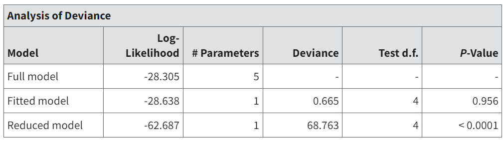
Figure 81. Analysis of Deviance table for MLE Dichotomous.
The Analysis of Deviance table displays three log-likelihood values.
The full model posits a separate and independent probability of response for each dose group. There is no dose-response function constraining those probabilities. The log-likelihood displayed is the maximum that could ever be achieved for the given dataset. The number of parameters for the full model is equal to the number of dose groups (each has its own, independent probability parameter).
The maximum log-likelihood value obtainable for the model under consideration. It corresponds to the model with the parameters set equal to the values shown in Individual Dichotomous Models and their Respective Parameters. The number of parameters equals the number of parameters in that table that are not reported as Bounded.
The maximum log-likelihood obtainable if one assumed that the same probability of response applied to all the dose groups, i.e., no difference in response over the dose levels. There is only 1 parameter for the reduced model, i.e., the assumed constant probability of response.
Associated with each of these three models are three values: Deviance, degrees of freedom (Test d.f.), and P-value.
The Deviance is twice the difference between the fitted or reduced model and the full model log-likelihood values. This Deviance is another goodness-of-fit metric: if the Deviance is small, then the smaller model (i.e., the fitted or reduced model) describes the data nearly as well as the full model does.
Deviance is approximately a Chi-square random variable with degrees of freedom specified by Test d.f., which is the difference in the number of parameters for the two models being compared.
The P-Value reflects the use of this Chi-square approximation to assess significance of the difference in fits. Larger deviances correspond to smaller p-values, so a small p-value indicates that the smaller model does not fit as well as the full model. The user may choose a rejection level (0.05 is common) to test if the model fit is appropriate.
For the fitted model, this is another measure of the fit of the model to the data.
For the reduced model, failure to reject that model (p-values greater than the rejection level chosen by the user) might lead the user to infer that there is no dose-related effect on response probabilities.
Plot and Error Bar Calculation
The graphical output (i.e., plot) is a visual depiction of the results of the modeling. Because plots, in general, were discussed in Graphs/Plots (All Endpoints), here we describe the one additional detail specific to the dichotomous models: computation of the error bars.
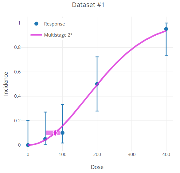
Figure 82. Dichotomous endpoint plot with error bars on the data points.
The error bars shown on the plots of dichotomous data (Figure 82.) are derived using a modification of the Wilson interval (based on the score statistic) but with a continuity correction method (Fleiss et al., 2003). The calculation finds the proportion, \(p_{i}\), such that
where
\(p\) is the observed proportion
\(n\) is the total number in the group in question, and
\(z = Z_{1 - \frac{\alpha}{2}}\) is the inverse standard Normal cumulative distribution function evaluated at \(1 - \frac{\alpha}{2}\)
This leads to equations for the lower and upper bounds of:
and
where \(q\ = \ 1 - p\).
The error bars shown in BMDS plots use alpha = 0.05 and so represent the 95% confidence intervals on the observed proportions (independent of model).
Mathematical Details for Models for Dichotomous Endpoints in Simple Designs
BMDS contains nine models for dichotomous endpoints as defined below.
Individual Dichotomous Models and their Respective Parameters
Model Form
Parameters
\(g\) = background
\(\beta_{j}\) = dose coefficients
Parameter Constraints
\(0\ \leq \ g\ < \ 1\)
\(n\ \leq \ 23\)
\(0\ < \beta < \ 10,000\)
User Parameter Restriction Options
Can restrict all \(\beta\) coefficients to \(leq\) 0. Doing so will guarantee that the multistage model will be either perfectly flat or always increasing.
Per EPA Technical Guidance (2012), when the Multistage model is used for cancer analyses (e.g., in Multitumor analyses) all \(\beta\) coefficients are restricted to be non-negative.
Model Form
Parameters
\(g\) = background
\(\alpha\) = power
\(\beta\) = slope
Parameter Constraints
\(0\ \leq \ g\ < \ 1\)
\(0\ < \ \alpha\ \leq \ 18\)
\(0\ < \ \beta < \ 100\)
User Parameter Restriction Options
\(1\ \leq \ \alpha\)
Notes
The Quantal Linear model results from setting \(\alpha\) = 1.
Model Form
Parameters
\(g\) = background
\(\alpha\) = power
\(\beta\) = slope
Parameter Constraints
\(0\ \leq \ g\ < \ 1\)
\(0.2\ < \ \alpha\ \leq \ 18\)
\(0\ < \ \beta\ < 100\)
User Parameter Restriction Options
\(1\ \leq \ \alpha\)
Notes
For the unrestricted Gamma model, \(\alpha >\) 0.2 for numerical reasons.
Model Form
Parameters
\(\alpha\) = intercept
\(\beta\) = slope
Parameter Constraints
\(- 18 < \alpha < 18\)
\(0 < \ \beta\ < 100\)
User Parameter Restriction Options
None.
Model Form
Parameters
\(g\) = background
\(\alpha\) = power
\(\beta\) = slope
Parameter Constraints
\(0\ \leq \ g\ < \ 1\)
\(- 18\ < \ \alpha\ \leq \ 18\)
\(0\ < \ \beta < 18\)
User Parameter Restriction Options
\(1\ \leq \beta\)
Model Form
where
\(\Phi(x) = \int_{- \infty}^{x}{\phi(t)dt}\)
and
\(\phi(t) = \ \frac{1}{\sqrt{2\pi}}e^{\frac{- t^{2}}{2}}\)
Parameters
\(\alpha\) = intercept
\(\beta\) = slope
Parameter Constraints
\(- 18 < \alpha < 18\)
\(0\ < \ \beta < 18\)
User Parameter Restriction Options
None.
Notes
\(\Phi\) is the standard Normal cumulative distribution function, \(\phi\) is the standard Normal density function.
Model Form
where
\(\Phi(x) = \int_{- \infty}^{x}{\phi(t)dt}\)
and
\(\phi(t) = \ \frac{1}{\sqrt{2\pi}}e^{\frac{- t^{2}}{2}}\)
Parameters
\(g\) = background
\(\alpha\) = intercept
\(\beta\) = slope
Parameter Constraints
\(0\ \leq \ g\ < \ 1\)
\(- 18\ \leq \alpha < 18\)
\(0\ < \ \beta\ \leq 18\)
User Parameter Restriction Options
\(1\ \leq \ \beta\)
Notes
For the log-probit model, the slope of the model will always approach zero as dose approaches zero regardless of the restriction on \(\beta\). However, for some relatively low doses (perhaps less than those corresponding to the BMR), the slope can be quite steep depending on the data and parameter estimates. In such cases, the BMDL estimate may be relatively low or perhaps NA if the steepness of the slope causes convergence problems as the BMDL estimate approaches zero.
Model Form
Parameters
\(g\) = background
\(v\) = maximum extra risk
\(\alpha\) = intercept
\(\beta\) = slope
Parameter Constraints
\(0\ \leq \ g\ < \ 1\)
\(- 18\ < \ v\ \leq 18\)
\(- 18\ < \alpha\ \leq 18\)
\(0\ < \ \beta\ \leq 18\)
User Parameter Restriction Options
\(1\ \leq \ \beta\)
Note
The upper bound for the power parameter in some of the models, and the slope parameter for some of the other models, has been set to 18. That value was selected because it represents a very high degree of curvature that should accommodate almost every dataset, even ones with very (or absolutely) flat dose-response at low doses followed by a very steep dose-response at higher doses.
If such parameter values are reported to be equal to 18 and/or the estimate in question is reported as Bounded (see the description of the output from dichotomous model runs in Analysis of Deviance Table), the parameter estimates are maximum likelihood estimates only in the restricted sense that the parameter in question has been assigned a value and the other parameters are MLEs conditional on that assigned value. Such model results are not strictly comparable with others in terms of AIC. In such a case, the BMD and BMDL could depend on the choice of power parameter; thus, sensitivity analysis is recommended if one intends to rely on the reported BMD or BMDL.
Note
The model descriptions above present the background parameter constraints on the logit scale, which is the form in which BMDS uses these constraints for calculation. The constraints are input into the software on the real number scale, with values of -18/18 for the MLE model and -20/20 for the Bayesian model minimum/maximum. The software then performs a logit transformation on these values. The background parameter values output by BMDS in the results will have a range of 0 to the maximum dose for each model.
Likelihood Function
The non-Bayesian dichotomous models are fit using maximum likelihood methods. This section describes the likelihood function used to fit the dichotomous models.
Suppose the dataset has G dose groups with doses:
The total numbers of observations and numbers of responders in each dose group are
and, respectively,
The distribution of \(n_{i}\) is assumed to be binomial with probability
where \(\theta\) is a vector of dose-response model parameters (see Individual Dichotomous Models and their Respective Parameters). Then the log-likelihood function \(LL\) can be written as
where
This expression ignores a constant term that is independent of the parameter vector values and so does not affect estimation of those parameters.
AIC and Model Comparisons
The Akaike Information Criterion (AIC) (Akaike, 1973) can be used to compare different models fit (by the same fitting method, e.g., by maximizing the likelihood) to the same dataset. The AIC is a statistic that depends on the value of LL (the log-likelihood function; see the previous section) and the number of estimated parameters, p:
Note
The AICs for the dichotomous endpoints ignore the parameter-independent term, because LL as defined in the previous section ignores that term. This differs from the case of the continuous endpoints, where the parameter-independent term was not ignored, because its value depended on the assumed underlying data distribution (Normal or Lognormal). For dichotomous endpoints, there is only one assumed distribution for the counts of responders (the Binomial distribution), so the parameter-independent term has no effect and therefore can be ignored.
The AIC balances the goals of getting the highest LL value possible while being parsimonious with respect to the number of parameters needed to achieve a high LL value. Since the equation for AIC has a negative multiplier for LL (which one wants to be greater) and positive multiplier for p (which one wants to be as small as possible and still get “good fit”), a model with a smaller value of AIC than other models is presumed to be the better model on the basis of AIC. Although such methods are not exact, they can provide useful guidance in model selection.
In the current version of BMDS, the number of estimated parameters includes only those that have not been estimated to equal a bounding value, either from the model-imposed constraints or user-imposed restrictions. For more details, see Individual Dichotomous Models and their Respective Parameters.
Note
The parameter counting process may or may not be reasonable, depending on the boundary value that a parameter in question hits.
For example, if the power parameter in a model hits (i.e., is estimated to be equal to) the upper bound of 18, it would usually be the case that one would want to count that parameter as one that is estimated, but BMDS does not do that.
For this reason, the user is apprised to carefully consider the cases where parameter bounds have been hit and to consider the implications for issues such as model comparison and model selection.
BMD Computation
The BMD is computed as a function of the parameters of the model under consideration (see Individual Dichotomous Models and their Respective Parameters). Solutions for the BMD for all the dichotomous models are shown below.
Calculation of the BMD for the Individual Dichotomous Models
There is no general analytical form for the BMD in terms of the BMR and the estimated model parameters for the multistage model. Instead, the BMD is the root of the equation
\(\beta_{1}BMD+\ldots{+ \ \beta}_{n}BMD^{n} + \ln(1-A) = 0\)
where
\(A = \left\{\begin{array}{r}BMR\ extra \ risk \\ \\ \frac{BMR}{1-g}\ added\ risk \end{array} \right.\\\)
\(BMD = \left\{\begin{array}{r}\left\lbrack \frac{- ln(1-BMR)}{\beta} \right\rbrack^{\frac{1}{\alpha}}\ extra\ risk \\ \\ \left\lbrack \frac{- ln(1 - \frac{BMR}{1-g})}{\beta} \right\rbrack^{\frac{1}{\alpha}}\ added\ risk \end{array} \right.\\\)
Let
\(G(x;\alpha) = \frac{1}{\Gamma(\alpha)}\int_{0}^{x}{t^{\alpha -1}e^{-t}dt}\)
be the incomplete Gamma function and
\(G^{-1}( \bullet ;\ \alpha)\)
be its inverse function. Then
\(BMD = \left\{\begin{array}{r}\frac{G^{-1}(BMR;\alpha)}{\beta}\ extra\ risk \\ \frac{G^{-1}(\frac{BMR}{1-g};\alpha)}{\beta}\ added\ risk \end{array} \right.\\\)
\(BMD = \frac{ ln(\frac{1-Z}{1 + Z \times e^{-\alpha}})}{\beta}\)
where
\(Z = \left\{ \begin{array}{r}BMR\ extra\ risk \\ \\ BMR \times \frac{1 + e^{- \alpha}}{e^{- \alpha}}\ added\ risk \end{array} \right.\\\)
\(\ln(BMD) = \left\{ \begin{array}{r}\frac{\ln\left( \frac{BMR}{1-BMR} \right) - \alpha}{\beta}\ extra\ risk \\ \\ \frac{\ln\left( \frac{BMR}{1 - g - BMR} \right) - \alpha}{\beta}\ added\ risk \end{array} \right.\\\)
\(BMD = \left\{ \begin{array}{r}\frac{\Phi^{-1}\left( BMR\left\lbrack 1-\Phi(\alpha) \right\rbrack + \Phi(\alpha) \right) - \alpha}{\beta}\ extra\ risk \\ \\ \frac{\Phi^{- 1}\left( BMR + \Phi(\alpha) \right) - \alpha}{\beta}\ added\ risk \end{array} \right.\\\)
\(ln(BMD) = \left\{ \begin{array}{r}\frac{\Phi^{- 1}(BMR) - \alpha}{\beta}\ extra\ risk \\ \\ \frac{\Phi^{- 1}\frac{BMR}{1 - g} - \alpha}{\beta}\ added\ risk\end{array} \right.\\\)
\(BMD = \left\{ \begin{array}{r} e\frac{- \alpha - \log\left( - \frac{BMR - v + gv}{BMR} \right)}{\beta}\ extra\ risk \\ \\ e\frac{- \alpha - \log\left( - \frac{BMR - v + gv- BMRgv}{BMR( - 1 + gv)} \right)}{\beta}\ added\ risk\end{array} \right.\\\)
Note
All models represented here use the same model forms as presented in Individual Dichotomous Models and their Respective Parameters. The BMR is the value specified by the user to correspond to the risk level of interest (see BMR).
BMDL and BMDU Computation
BMDS currently calculates one-sided confidence intervals, in accordance with current BMD practice. The general approach to computing the confidence limits for the BMD (called the BMDL and BMDU here) is the same for all the models in BMDS, and is based on the asymptotic distribution of the likelihood ratio (Crump and Howe, 1985). Two different specific approaches are followed in these models.
For the Multistage model, it is impractical to explicitly reparameterize the dose-response model function to allow BMD to appear as an explicit parameter. For these models, the BMR equation is used as a non-linear constraint, and the minimum value of BMD is determined such that the resulting log-likelihood is less than that at the maximum likelihood estimates by exactly
For the remaining models, the equations that define the benchmark response in terms of the benchmark dose and the dose-response model (Calculation of the BMD for the Individual Dichotomous Models) are solved for one of the model parameters. The resulting expression is substituted back into the model equations, with the effect of reparameterizing the model so that BMD appears explicitly as a parameter. A value for BMD is then found such that, when the remaining parameters are varied to maximize the likelihood, the resulting log-likelihood is less than that at the maximum likelihood estimates by exactly
In all cases, the additional constraints specify that the BMDL be less than the BMD and the BMDU be greater than the BMD.
Rao-Scott Transformation for Modeling Summary Dichotomous Developmental Data
The Rao-Scott transformation is an approach, described in Fox et al., 2017, to model dichotomous developmental data when only summary level dose-response data is available. The transformation works by scaling dose-level incidence and sample size data by a variable called the design effect in order to approximate the intralitter correlation that occurs due to the clustered study design of developmental toxicity studies.
Note
If individual-level developmental toxicity data are available for modeling, see Nested Dichotomous Endpoints for details on the usage of the nested dichotomous models available in BMDS Online.
To access the Rao-Scott transformation:
Select Dichotomous on the Settings tab.
Select the Data tab.
Beneath the data table, select the link for Rao-Scott Transformation
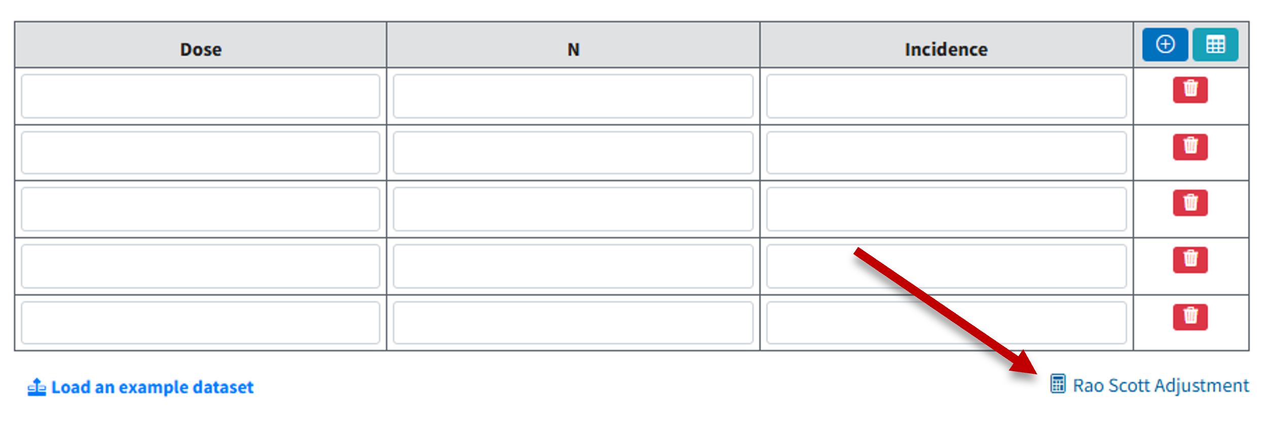
Figure 83. With Dichotomous as the model type, BMDS Online displays a Rao-Scott transformation link under the data table.
Selecting the link displays the Rao-Scott transformation page, where the user can enter their data and specify settings. Users can copy and paste data from a CSV file or an Excel sheet into the Dataset text field.
Under the Dataset table:
Select the load link to have BMDS Online load an example dataset.
The dataset used for the Rao-Scott transformation should have the same structure as regular dichotomous data and should have the following columns in this sequence:
Dose Numeric value of the dose group
N Numeric value for the number of fetuses (irrespective of litter membership) per dose group
Incidence Numeric value for the number of affected fetuses (irrespective of litter membership) per dose group
Additionally, users will need to select the species that corresponds to their dose-response data; currently options for species are limited to rat, mouse, and rabbit.
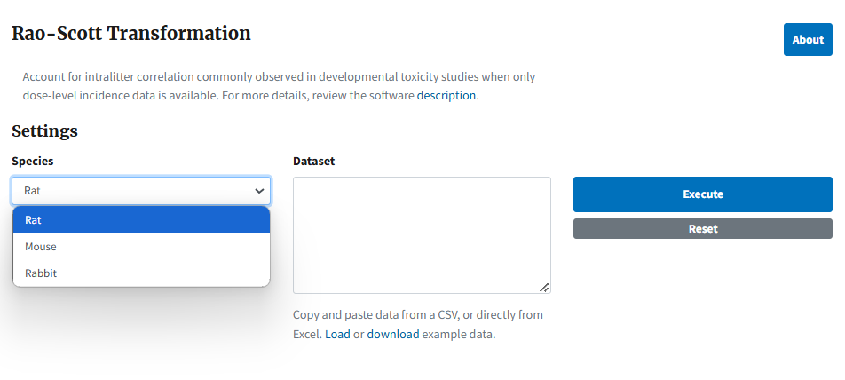
Figure 84. The Rao-Scott transformation page, with an example dataset loaded
Select the Execute button to run the analysis. BMDS Online extends the Rao-Scott transformation page with the following outputs:
A summary table of the original and adjusted data
Plots of the original and adjusted values for both the total number of fetuses and number of affected fetuses per dose group
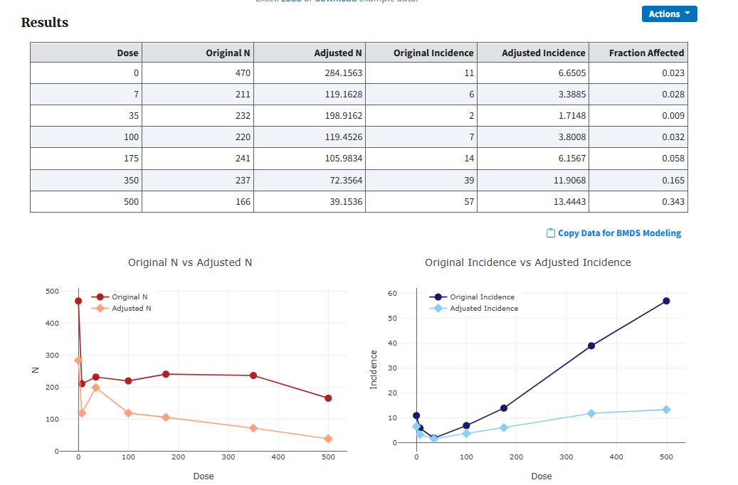
Figure 85. Result of running a Rao-Scott transformation, with summary table of results and plots of adjusted vs original values
The Copy Data for BMDS Modeling link copies the summary table data to the clipboard. From there, the user can return to their Dichotomous analysis, return to the data table, select the Load dataset from Excel button, and paste the clipboard contents to create a new dataset. Or they can paste the clipboard contents into Excel for further analysis.
From the Actions drop down menu, users can download the Rao-Scott adjusted data or create a Word report documenting the Rao-Scott transformation. This Word report will recapitulate the summary table and plots previously displayed in the browser window and will additionally report the actual values of the design effect estimated from the entered unadjusted data and the Rao-Scott regression parameter values.
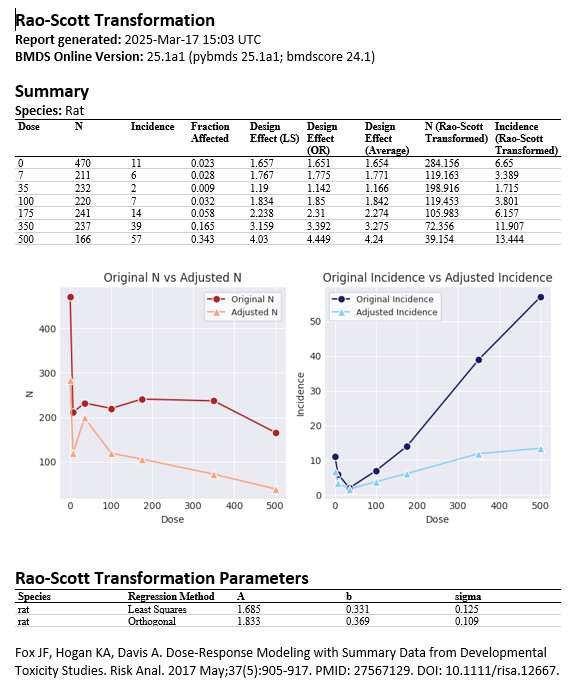
Figure 86. Rao-Scott transformation Word report, with summary table of results, plots of original vs adjusted values, and Rao-Scott transformation regression parameter values
More on the Rao-Scott Transformation
For dose-response analyses of dichotomous developmental toxicity studies, the proper approach is to model individual animal data (i.e., litter data for individual dams) in order to account for the tendency of pups from one litter to respond more alike one another than pups from other litters. This behavior is commonly termed the litter effect or intralitter correlation (see Nested Dichotomous Endpoints for more details).
However, it is frequently the case that dose-response modelers will be modeling data reported in the peer-reviewed literature and it is rarely the case that individual litter data is reported in peer-reviewed articles or provided as supplemental materials. Instead, peer-reviewed articles typically report the dose-level summary data: the total number of fetuses and the number of fetuses responding per dose group, but not information on how many fetuses from each litter were affected. When dose-level summary data is reported, it is impossible to account for the presence of intralitter correlations when conducting benchmark dose analyses of dichotomous data.
If summary developmental data (i.e., dose-level fetal Ns and incidence) were modeled with regular dichotomous models without accounting for the litter effect, misleading modeling results can occur, including incorrect perception of high precision, smaller p-values than warranted, and narrower confidence intervals. These effects are due to the fact that the “true” variance would be underestimated if clustering is ignored because the observations are correlated. The most consequential effect would be that larger, less health-protective, BMDLs would be estimated given that the confidence interval around the BMD would be narrower.
Ultimately, ignoring litter effects results in biased estimates from dose-response models. Therefore, alternative statistical approaches are necessary in order to use summary statistics while also accounting for intralitter correlation. As reported in Fox et al., 2017, multiple statistical studies have researched the concept of the design effect, \(D\), as a strategy to reduce overdispersion arising from clustered study design via a simple dose-response transformation. The core concept is that correlated data can be transformed via scaling and then modeled with standard dichotomous models as if they were not correlated. As Fox et al., 2017 reports, the design effect is related approximately to intralitter correlation \(\rho_{I}\) as \(D = \left\lbrack 1 + (n -1)\rho_{I} \right\rbrack\) in the special case that all litters have \(n\) offspring. More typically, a weighted average of litter size is used.
As described in Fox et al., 2017, \(D\) is the ratio of the variance for correlated, clustered data and the variance for uncorrelated binomial data, given both have the same average proportion of affected animals. An estimate of the proportion of affected fetuses, \(P_{f}=\frac{A_{f}}{N_{f}}\), where \(A_{f}\) is the number of affected fetuses and \(N_{f}\) is the total number of fetuses, is required by both measures of variance.
The estimated variance of a binomial proportion is the denominator for \(D\):
Whereas an estimate of the correct variance for the correlated data (based on a weighted sum of the squared deviations of litter proportions, \(p_{i}\) in the \(i^{th}\) litter, from \(P_{f}\)) is the numerator of \(D\):
where \(n_{i}\) is the number of offspring in the \(i^{th}\) litter and \(m\) is the number of litters.
In order to apply the Rao-Scott transformation, both the numerator and denominator of a dose-level proportion are divided by \(D\). This results in what can be described as the effective sample size \(\left({N_{f}}_{RS} = \frac{N_{f}}{D}\right)\) and the effective affected fetuses \(\left({A_{f}}_{RS} = \frac{A_{f}}{D}\right)\).
As can be seen in the equations above, the calculation of the design effect requires litter-level data given the need to know \(p_{i}\) for each litter and that it thus cannot be calculated directly from dose-group-level data. In order to provide BMDS users an approach to approximate \(D\) for summary data, Fox et al., 2017 conducted an analysis of 55 developmental toxicity studies for which individual level data were available and used the regression equation \(\ln(D) = a + b \times\ln(P_{f})\) to establish the relationship between \(D\) and \(P_{f}\) for studies that used either rats, mice, or rabbits as their test species. This analysis used both least-squares and orthogonal regression. The table below reports the species-specific regression coefficients for the established relationship between \(D\) and \(P_{f}\).
Species |
Method |
\(n\), Studies |
\(n\), Dose Groups |
\(a\) |
\(b\) |
\(\sigma_{res}^{2}\) |
|---|---|---|---|---|---|---|
Mice |
LS |
21 |
88 |
1.5938 |
0.2866 |
0.2078 |
Mice |
OR |
21 |
88 |
1.6943 |
0.3132 |
0.1863 |
Rats |
LS |
25 |
101 |
1.6852 |
0.3310 |
0.1248 |
Rats |
OR |
25 |
101 |
1.8327 |
0.3690 |
0.1090 |
Rabbits |
LS |
10 |
43 |
1.0582 |
0.2397 |
0.1452 |
Rabbits |
OR |
10 |
43 |
1.1477 |
0.2739 |
0.1299 |
From these regression coefficients, the design effect can be calculated as \(D = e^{\left\lbrack a + b \times \ln(P_{f})+0.5\sigma_{res}^{2} \right\rbrack}\). Given there is no strong methodological preference using the design effect calculated using linear least squares regression (\(D_{LS}\)) vs the design effect calculated using orthogonal regression (\(D_{OR}\)), by practice the design effect estimated using these two regression approaches is averaged to generate the average design effect (\(D_{average}\)) actually used in the scaling of \(N_{f}\) and \(A_{f}\). An example calculation is provided below for a hypothetical developmental study using mice.
Dose |
\(N_{f}\) |
\(A_{f}\) |
\(P_{f}\) |
\(D_{LS}\) |
\(D_{OR}\) |
\(D_{average}\) |
\({N_{f}}_{RS}\) |
\({A_{f}}_{RS}\) |
\({P_{f}}_{RS}\) |
|---|---|---|---|---|---|---|---|---|---|
0 |
121 |
1 |
0.0083 |
1.1737 |
1.1247 |
1.1493 |
105.287 |
0.870 |
0.0083 |
25 |
116 |
7 |
0.0604 |
2.2666 |
2.3424 |
2.3045 |
50.337 |
3.038 |
0.0604 |
50 |
114 |
24 |
0.2106 |
3.4276 |
3.7145 |
3.5710 |
31.924 |
6.721 |
0.2105 |
100 |
105 |
52 |
0.4952 |
4.5494 |
5.0932 |
4.8213 |
21.778 |
10.786 |
0.4952 |
For example, using the 25 ppm dose group as an example, the Rao-Scott transformed N (\({N_{f}}_{RS}\)) would be calculated as:
Design effect using LS regression coefficients: \(D_{LS}= e^{\left\lbrack 1.6852 + 0.3310 \times \ln(0.0604) + 0.5 \times 0.1248 \right\rbrack} = 2.2666\)
Design effect using OR regression coefficients: \(D_{OR}= e^{\left\lbrack 1.8327 + 0.3690 \times \ln(0.0604) + 0.5 \times 0.1090 \right\rbrack} = 2.3424\)
Average design effect: \(D_{average} = \frac{2.2666 + 2.3424}{2} = 2.3045\)
Rao-Scott transformed N: \({N_{f}}_{RS} = \frac{116}{2.3045} = 50.337\)
For modeling the transformed data in BMDS, the values in the \({N_{f}}_{RS}\) and \({A_{f}}_{RS}\) column would be entered as the modeling inputs. Note that the original \(P_{f}\) and Rao-Scott transformed \({P_{f}}_{RS}\) values are identical.
The ultimate consequence of the Rao-Scott transformation will be the estimation of wider confidence intervals for the BMD, and thus lower BMDLs. This is the consequence of the transformation that is most important as the lower BMDLs of the Rao-Scott transformed fetal incidence data approximate the BMDLs that would be estimated had individual-level data been modeled with a nested dichotomous model. Fox et al., 2017 compared multiple approaches for accounting for intralitter correlation using summary level data (e.g., setting \(D\) equal to a set value, setting \(D = \frac{N_{f}}{N_{L}}\), modeling average proportion affected as a continuous variable, or modeling the proportion of litters responding) and saw that using the design effects estimated from the historical data regressions (i.e., the method described above) resulted in BMDLs that were most equivalent to those achieved modeling individual-level data.
Trend Test for Dichotomous Data
The Cochran-Armitage trend test allows users to test for trends in binomial proportions across different levels of a single variable. In the case of dichotomous dose-response data, the number of responses divided by the total number of subjects exposed represents the binomial proportion, which is tested across the different doses. Here, dose is treated as an ordinal variable, and thus the test depends only on the order of the doses, not their numerical values. The Cochran-Armitage trend test in pybmds automatically computes both the asymptotic and conditional exact p-values for testing the presences of a monotonic trend in incidence rations across increasing dose groups.
The asymptotic p-value is based on a normal approximation of the linear trend statistic proposed by Cochran (1954) and Armitage (1954). The exact one-sided p-value for the Cochran-Armitage trend test uses a special case of the linear rank test algorithm by Mehta, Patel, and Tsiastis (1992).
The null hypothesis for the Cochran-Armitage test is that the binomial proportion of the responses is the same across all levels of the ordinal dose variable; p-values less than the alpha level (normally 0.05) indicate that a monotonic trend does exist in the data.
Note
At this time, the Cochran-Armitage trend test is only available in pybmds (version 25.2). See pybmds Documentation for examples of usage