Simulation results#
Simulation results are stored in a results object which contains:
Timestamp when the results were created
Network name
Node results
Link results
As shown in the Hydraulic simulation and Water quality simulation sections, simulations results can be generated using the EpanetSimulator as follows (similar methods are used to generate results using the WNTRSimulator):
>>> import wntr

>>> wn = wntr.network.WaterNetworkModel('Net3')
>>> sim = wntr.sim.EpanetSimulator(wn)
>>> results = sim.run_sim()
The node and link results are dictionaries of pandas DataFrames. Each dictionary is a key:value pair, where the key is a result attribute (e.g., node demand, link flowrate) and the value is a DataFrame. DataFrames are indexed by timestep (in seconds from the start of the simulation) with columns that are labeled using node or link names.
The use of pandas facilitates a comprehensive set of time series analysis options that can be used to evaluate results. For more information on pandas, see https://pandas.pydata.org.
Conceptually, DataFrames can be visualized as blocks of data with 2 axis, as shown in Figure 14.
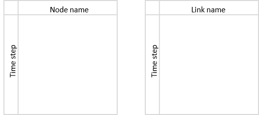
Figure 14 Conceptual representation of DataFrames used to store simulation results.#
Node results include DataFrames for each of the following attributes:
Demand
Leak demand (only when the WNTRSimulator is used, see the Note below)
Head
Pressure
Quality (only when the EpanetSimulator is used. Water age, tracer percent, or chemical concentration is stored, depending on the mode of water quality analysis)
For example, node results generated with the EpanetSimulator have the following keys:
>>> node_keys = results.node.keys()
>>> print(node_keys)
dict_keys(['demand', 'head', 'pressure', 'quality'])
Note
When using the WNTRSimulator, leak demand is distinct from demand, therefore total demand = demand + leak demand. When using the EpanetSimulator, emitters are included in demand, therefore total demand = demand.
Link results include DataFrames for each of the following attributes:
Velocity
Flowrate
Setting
Status (0 indicates closed pipe/pump/valve, 1 indicates open pipe/pump/valve, 2 indicates active valve)
Headloss (only when the EpanetSimulator is used)
Friction factor (only when the EpanetSimulator is used)
Reaction rate (only when the EpanetSimulator is used)
Link quality (only when the EpanetSimulator is used)
The link results that are only accessible from the EpanetSimulator could be included in the WNTRSimulator in a future release. For example, link results generated with the EpanetSimulator have the following keys:
>>> link_keys = results.link.keys()
>>> print(link_keys)
dict_keys(['flowrate', 'friction_factor', 'headloss', 'quality', 'reaction_rate', 'setting', 'status', 'velocity'])
To access node pressure over all nodes and times:
>>> pressure = results.node['pressure']
DataFrames can be sliced to extract specific information. For example, to access the pressure at node ‘123’ over all times (the “:” notation returns all variables along the specified axis, “head()” returns the first 5 rows, values displayed to 2 decimal places):
>>> pressure_at_node123 = pressure.loc[:,'123']
>>> print(pressure_at_node123.head())
0        47.08
3600     47.95
7200     48.75
10800    49.13
14400    50.38
Name: 123, dtype: float32
To access the pressure at time 3600 over all nodes (values displayed to 2 decimal places):
>>> pressure_at_1hr = pressure.loc[3600,:]
>>> print(pressure_at_1hr.head())
name
10    28.25
15    28.89
20     9.10
35    41.51
40     4.19
Name: 3600, dtype: float32
Data can be plotted as a time series, as shown in Figure 15:
>>> ax = pressure_at_node123.plot()
>>> text = ax.set_xlabel("Time (s)")
>>> text = ax.set_ylabel("Pressure (m)")
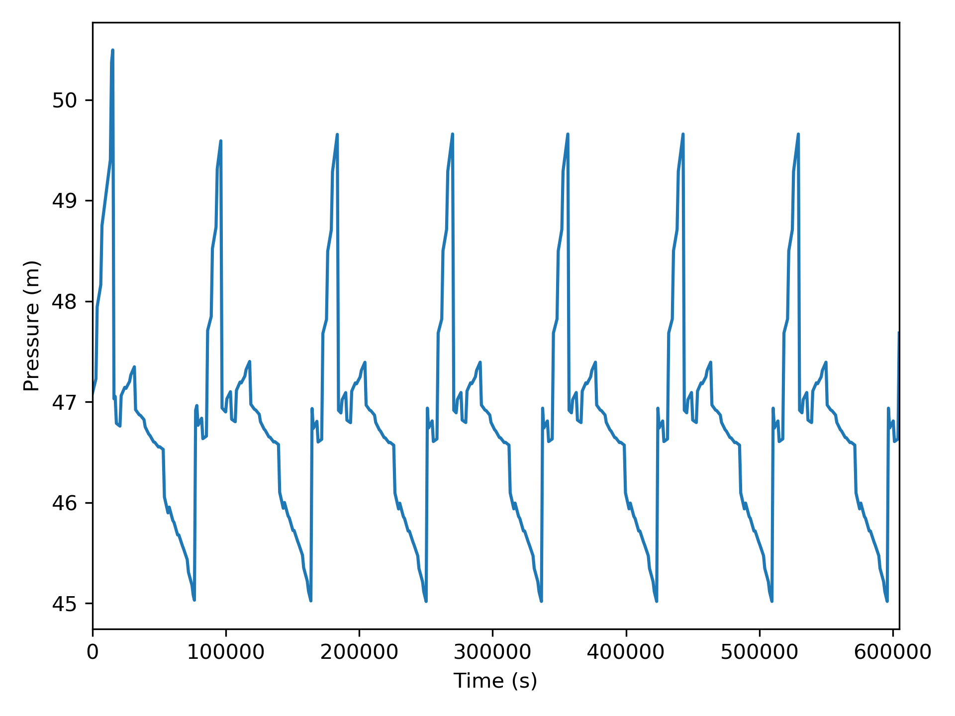
Figure 15 Time series graphic showing pressure at a node.#
Data can also be plotted on the water network model, as shown in Figure 16.
Note that the plot_network function returns matplotlib objects
for the network nodes and edges, which can be further customized by the user.
In this figure, the node pressure at 1 hr is plotted on the network. Link attributes can be
plotted in a similar manner.
>>> ax = wntr.graphics.plot_network(wn, node_attribute=pressure_at_1hr,
...    node_range=[30,55], node_colorbar_label='Pressure (m)')
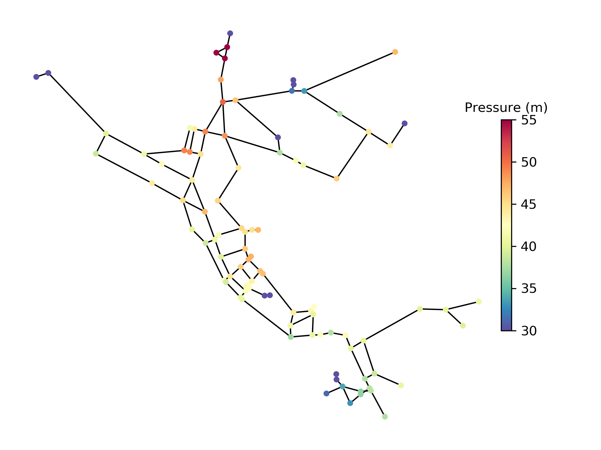
Figure 16 Network graphic showing pressure at 1 hour.#
Network and time series graphics can be customized to add titles, legends, axis labels, and/or subplots.
Pandas includes methods to write DataFrames to the following file formats:
Microsoft Excel (xlsx)
Comma-separated values (CSV)
Hierarchical Data Format (HDF)
JavaScript Object Notation (JSON)
Structured Query Language (SQL)
For example, DataFrames can be saved to Excel files using:
>>> pressure.to_excel('pressure.xlsx')
Note
The Pandas method to_excel requires the Python package openpyxl [8], which is an optional dependency of WNTR.
Water quality results#
Water quality metrics are stored under the ‘quality’ key of the node and link results if the EpanetSimulator is used. The units of the quality results depend on the quality parameter that is used (see _water_quality_simulation) and can be the age, concentration, or the fraction of water that belongs to a tracer. If the parameter is set to ‘NONE’, then the quality results will be zero.
The quality of a link is equal to the average across the length of the link. The quality at a node is the instantaneous value.
When using the EPANET-MSX water quality model, each species is given its own key in the node and link results objects, and the ‘quality’ results still references the EPANET water quality results.