Geospatial capabilities#
The junctions, tanks, reservoirs, pipes, pumps, and valves in a WaterNetworkModel
can be converted to GeoPandas GeoDataFrames as described in Model I/O.
The GeoDataFrames can be used
directly within WNTR,
with geospatial Python packages such as GeoPandas and Shapely, and saved to GeoJSON and Shapefiles for use
in GIS platforms.
Open source GIS platforms include QGIS and GRASS GIS.
The following section describes capabilities in WTNR that use GeoPandas GeoDataFrames.
Note
Functions that use GeoDataFrames require the Python package geopandas [15] and rtree [28], and functions that use raster files require the Python package rasterio. All three are optional dependencies of WNTR. Note that shapely is installed with geopandas.
The following examples use a water network generated from Net1.inp.
The snap and intersect examples
also use additional GIS data stored in the
examples/data directory.
For simplicity, the examples in this section assume that all network and data coordinates are in the EPSG:4326 coordinate reference system (CRS). Note that EPANET does not have a standard or default coordinate reference system. More information on setting and transforming CRS is included in Coordinate reference system.
>>> import wntr

>>> wn = wntr.network.WaterNetworkModel('Net1')
Water network GIS data#
The to_gis function is used to
create a collection of GeoDataFrames from a WaterNetworkModel.
The collection of GeoDataFrames is stored in a WaterNetworkGIS object
which contains a GeoDataFrame
for each of the following model components:
junctions
tanks
reservoirs
pipes
pumps
valves
Note that patterns, curves, sources, controls, and options are not stored in the GeoDataFrame representation.
>>> wn_gis = wntr.network.to_gis(wn)
Individual GeoDataFrames are obtained as follows (Note that the example network, Net1, has no valves and thus the GeoDataFrame for valves is empty).
>>> wn_gis.junctions
>>> wn_gis.tanks
>>> wn_gis.reservoirs
>>> wn_gis.pipes
>>> wn_gis.pumps
>>> wn_gis.valves
For example, the junctions GeoDataFrame contains the following information:
>>> print(wn_gis.junctions.head())
      base_demand demand_pattern  elevation  initial_quality demand_category       geometry
name
10          0.000              1    216.408        5.000e-04            None  POINT (20 70)
11          0.009              1    216.408        5.000e-04            None  POINT (30 70)
12          0.009              1    213.360        5.000e-04            None  POINT (50 70)
13          0.006              1    211.836        5.000e-04            None  POINT (70 70)
21          0.009              1    213.360        5.000e-04            None  POINT (30 40)
Each GeoDataFrame contains attributes and geometry:
Attributes#
A GeoDataFrame contains attributes that are generated from the WaterNetworkModel dictionary representation. However, the GeoDataFrame only includes attributes that are stored as numerical values or strings (such as junction node type and elevation). Attributes that are stored as lists or other objects (such as demand timeseries) are not included in the GeoDataFrame. The index for each GeoDataFrame is the model component name.
Additional attributes can be added to the GeoDataFrames using the
add_node_attributesandadd_link_attributesmethods. Additional attributes, such as simulation results or a resilience metric, can be used in further analysis and visualization.The following example adds the simulated pressure at hour 1 to the water network GIS data (which includes pressure at junctions, tanks, and reservoirs).
 >>> sim = wntr.sim.EpanetSimulator(wn)
 >>> results = sim.run_sim()
 >>> wn_gis.add_node_attributes(results.node['pressure'].loc[3600,:],
 ...     'Pressure_1hr')
Attributes can also be added directly to individual GeoDataFrames, as shown below.
>>> wn_gis.junctions['new attribute'] = 10
Geometry#
Each GeoDataFrame also contains a geometry column which contains geometric objects commonly used in geospatial analysis. Table 11 includes water network model components and the geometry type that defines each component. Geometry types include
shapely.geometry.Point,shapely.geometry.LineString, andshapely.geometry.MultiLineString. A few components can be defined using multiple types:
Pumps and valves can be stored as lines (default) or points. While pumps are defined as lines within WNTR (and EPANET), converting the geometry to points can be useful for geospatial analysis and visualization. The following example stores pumps and valves as points.
>>> wn_gis = wntr.network.to_gis(wn, pumps_as_points=True,
...     valves_as_points=True)
Pipes that do not contain vertices, interior vertex points that allow the visual depiction of curved pipes, are stored as a LineString while pipes that contain vertices are stored as a MultiLineString.
Table 11 Geometry Types for Water Network Model Components# Water Network Model Component
Shapely Geometry Type
Junction
Point
Tank
Point
Reservoir
Point
Pipe
LineString or MultiLineString
Pump
LineString or Point
Valve
LineString or Point
A WaterNetworkGIS object can also be written to GeoJSON and Shapefiles using
the object’s write_geojson and
write_shapefile methods.
See Shapefile for more information on Shapefile format.
The GeoJSON and Shapefiles can be loaded into GIS platforms for further analysis and visualization.
An example of creating GeoJSON files from a WaterNetworkModel using the function write_geojson
is shown below.
>>> wn_gis.write_geojson('Net1')
This creates the following GeoJSON files for junctions, tanks, reservoirs, pipes, and pumps (Note that the example network, Net1, has no valves and thus the Net1_valves.geojson file is not created):
Net1_junctions.geojson
Net1_tanks.geojson
Net1_reservoirs.geojson
Net1_pipes.geojson
Net1_pumps.geojson
A WaterNetworkModel can also be created from a collection of GeoDataFrames using the function
from_gis as shown below.
>>> wn2 = wntr.network.from_gis(wn_gis)
Additional GIS data#
Additional GIS data can also be utilized within WNTR to add attributes to the water network model and analysis. Examples of these additional GIS datasets include:
Point geometries that could contain utility billing data, hydrant locations, isolation valve locations, or the location of emergency services. These geometries can be associated with points and lines in a water network model by snapping the point to the nearest component.
LineString or MultiLineString geometries that could contain street layout or earthquake fault lines. These geometries can be associated with points and lines in a water network model by finding the intersection.
Polygon geometries that could contain elevation, building footprints, zoning, land cover, hazard maps, census data, or demographics. These geometries can be associated with points and lines in a water network model by finding the intersection.
The snap and intersect examples below used additional GIS data stored in the examples/data directory.
Note, the GeoPandas read_file and to_file functions can be used to read/write external GeoJSON and Shapefiles in Python.
Coordinate reference system#
The coordinate reference system (CRS) of geospatial data is important to understand. CRSs can be geographic (e.g., latitude/longitude where the units are in degrees) or projected (e.g., Universal Transverse Mercator where units are in meters). GeoPandas includes documentation on managing projections at https://geopandas.org/en/stable/docs/user_guide/projections.html. Several important points on CRS are listed below.
The GeoPandas
set_crsandto_crsmethods can be used to set and transform the CRS of GeoDataFrames.The WNTR WaterNetworkGIS object also includes
set_crsandto_crsmethods to set and transform the CRS of the junctions, tanks, reservoirs, pipes, pumps, and valves GeoDataFrames.WNTR includes additional methods to modify coordinates on the WaterNetworkModel object, see Modify node coordinates for more information.
When converting a WaterNetworkModel into GeoDataFrames using
to_gisand when creating GeoJSON and Shapefiles from a WaterNetworkModel usingwrite_geojsonandwrite_shapefile, the user can specify a CRS for the node coordinates. This does NOT convert node coordinates to a different CRS. It only assigns a CRS to the data or file. By default, the CRS is not specified (and is set to None).The
snapandintersectfunctions described in the following sections require that datasets have the same CRS.Projected CRSs are preferred for more accurate distance calculations.
The following example reads a GeoJSON file and overrides the CRS to change it from EPSG:4326 to EPSG:3857. (Note, this does not change the coordinates in the geometry column.)
>>> import geopandas as gpd

>>> hydrant_data = gpd.read_file('data/Net1_hydrant_data.geojson')
>>> print(hydrant_data.crs)
EPSG:4326
>>> print(hydrant_data)
   demand           geometry
0    5000  POINT (48.2 37.2)
1    1500  POINT (71.8 68.3)
2    8000  POINT (51.2 71.1)

>>> hydrant_data = hydrant_data.set_crs('EPSG:3857', allow_override=True)
>>> print(hydrant_data.crs)
EPSG:3857
>>> print(hydrant_data)
   demand           geometry
0    5000  POINT (48.2 37.2)
1    1500  POINT (71.8 68.3)
2    8000  POINT (51.2 71.1)
The following example reads a GeoJSON file and transforms the CRS to EPSG:3857. (Note, this transforms the coordinates in the geometry column.)
>>> hydrant_data = gpd.read_file('data/Net1_hydrant_data.geojson')

>>> hydrant_data.to_crs('EPSG:3857', inplace=True)
>>> print(hydrant_data.crs)
EPSG:3857
>>> print(hydrant_data)
   demand                          geometry
0    5000   POINT (5365599.456 4467020.994)
1    1500  POINT (7992739.439 10536729.551)
2    8000  POINT (5699557.929 11436551.505)
The following example converts a WaterNetworkModel in EPSG:4326 coordinates into GeoDataFrames and then translates the GeoDataFrames coordinates to EPSG:3857.
>>> wn = wntr.network.WaterNetworkModel('Net1')

>>> wn_gis = wntr.network.to_gis(wn, crs='EPSG:4326')
>>> print(wn_gis.junctions.head())
      base_demand demand_pattern  elevation  initial_quality demand_category       geometry
name
10          0.000              1    216.408        5.000e-04            None  POINT (20 70)
11          0.009              1    216.408        5.000e-04            None  POINT (30 70)
12          0.009              1    213.360        5.000e-04            None  POINT (50 70)
13          0.006              1    211.836        5.000e-04            None  POINT (70 70)
21          0.009              1    213.360        5.000e-04            None  POINT (30 40)

>>> wn_gis.to_crs('EPSG:3857')
>>> print(wn_gis.junctions.head())
      base_demand demand_pattern  elevation  initial_quality demand_category                          geometry
name
10          0.000              1    216.408        5.000e-04            None  POINT (2226389.816 11068715.659)
11          0.009              1    216.408        5.000e-04            None  POINT (3339584.724 11068715.659)
12          0.009              1    213.360        5.000e-04            None   POINT (5565974.54 11068715.659)
13          0.006              1    211.836        5.000e-04            None  POINT (7792364.356 11068715.659)
21          0.009              1    213.360        5.000e-04            None    POINT (3339584.724 4865942.28)
Snap point geometries to the nearest point or line#
The snap function is used to find the nearest point or line to a set of points.
This functionality can be used to assign hydrants to junctions or assign isolation valves to pipes.
For example, when snapping point geometries in GeoDataFrame A to point or line geometries in GeoDataFrame B, the function returns the following information (one entry for each point in A):
Nearest point or line in B
Distance between original and snapped point
Coordinates of the snapped point
If B contains lines, the nearest endpoint along the nearest line
If B contains lines, the relative distance from the line’s start node (line position)
The network file, Net1.inp, in EPSG:4326 CRS is used in the example below. The additional GIS data in the GeoJSON format is also in EPSG:4326 CRS. See Coordinate reference system for more information.
>>> wn = wntr.network.WaterNetworkModel('Net1')
>>> wn_gis = wntr.network.to_gis(wn, crs='EPSG:4326')
Snap hydrants to junctions#
GIS data which include the network hydrant locations is useful in a resilience analysis. In particular,
this information identifies which junctions could have their demands increased to simulate the opening
of hydrants to fight fires or flush contaminated water out of the network, either of which could caused by a disaster scenario.
The following example highlights the process to snap hydrants to junctions. The example dataset of hydrant
locations is a GeoDataFrame with a geometry column that contains shapely.geometry.Point geometries and a
demand column that defines fire flow requirements.
The GeoPandas read_file method is used to read the GeoJSON file into a GeoDataFrame.
>>> import geopandas as gpd

>>> hydrant_data = gpd.read_file('data/Net1_hydrant_data.geojson')
>>> print(hydrant_data)
   demand           geometry
0    5000  POINT (48.2 37.2)
1    1500  POINT (71.8 68.3)
2    8000  POINT (51.2 71.1)
The following example uses the function snap to snap hydrant locations to the nearest junction
within a tolerance of 5.0 units (the tolerance is in the units of the GIS coordinate system).
>>> snapped_to_junctions = wntr.gis.snap(hydrant_data, wn_gis.junctions, tolerance=5.0)
>>> print(snapped_to_junctions)
  node  snap_distance       geometry
0   22          3.329  POINT (50 40)
1   13          2.476  POINT (70 70)
2   12          1.628  POINT (50 70)
The data, water network model, and snapped points can be plotted as follows. The resulting Figure 38 illustrates the hydrants snapped to the junctions in Net1.
>>> ax = hydrant_data.plot()
>>> ax = wntr.graphics.plot_network(wn,
...     node_attribute=snapped_to_junctions['node'].to_list(), ax=ax)
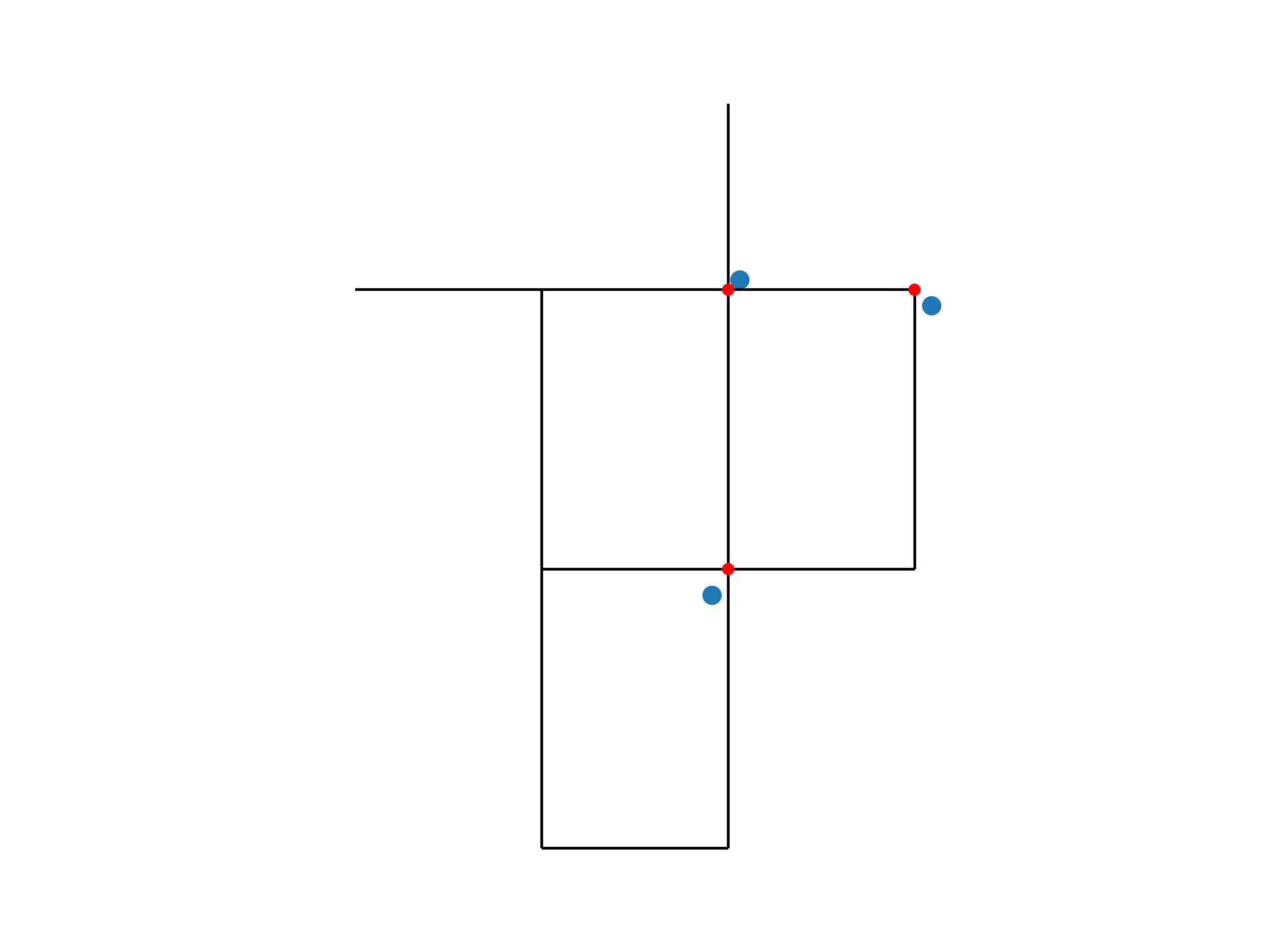
Figure 38 Net1 with example hydrants snapped to junctions, in which the larger blue circles are the hydrant locations and the smaller red circles are the associated junctions.#
By reversing the order of GeoDataFrames in the snap function, the nearest hydrant to each junction can also be identified. Note that the tolerance is increased to ensure all junctions are assigned a hydrant.
>>> snapped_to_hydrants = wntr.gis.snap(wn_gis.junctions, hydrant_data, tolerance=100.0)
>>> print(snapped_to_hydrants)
    node  snap_distance           geometry
10     2         31.219  POINT (51.2 71.1)
11     2         21.229  POINT (51.2 71.1)
12     2          1.628  POINT (51.2 71.1)
13     1          2.476  POINT (71.8 68.3)
21     0         18.414  POINT (48.2 37.2)
22     0          3.329  POINT (48.2 37.2)
23     0         21.979  POINT (48.2 37.2)
31     0         32.727  POINT (48.2 37.2)
32     0         27.259  POINT (48.2 37.2)
Snap valves to pipes#
GIS data of the network isolation valve locations can be used to identify which pipes to
close during a pipe break scenario. The following example highlights the process to snap valves to pipes.
The example dataset of valve locations is a GeoDataFrame with a geometry column that contains shapely.geometry.Point geometries.
>>> valve_data = gpd.read_file('data/Net1_valve_data.geojson')
>>> print(valve_data)
            geometry
0  POINT (56.5 41.5)
1  POINT (32.1 67.6)
2  POINT (52.7 86.3)
The following example uses the function snap to snap valve locations to the nearest pipe
within a tolerance of 5.0 degrees.
>>> snapped_to_pipes = wntr.gis.snap(valve_data, wn_gis.pipes, tolerance=5.0)
>>> print(snapped_to_pipes)
  link node  snap_distance  line_position         geometry
0   22   22            1.5          0.325  POINT (56.5 40)
1  111   11            2.1          0.080  POINT (30 67.6)
2  110    2            2.7          0.185  POINT (50 86.3)
The snapped locations can be used to define a Valve layer and then create network segments.
>>> valve_layer = snapped_to_pipes[['link', 'node']]
>>> G = wn.to_graph()
>>> node_segments, link_segments, segment_size = wntr.metrics.valve_segments(G,
...     valve_layer)
The data, water network model, and valve layer can be plotted as follows. The resulting Figure 39 illustrates the valve layer created by snapping points to lines in Net1.
>>> ax = valve_data.plot()
>>> ax = wntr.graphics.plot_valve_layer(wn, valve_layer, add_colorbar=False, ax=ax)
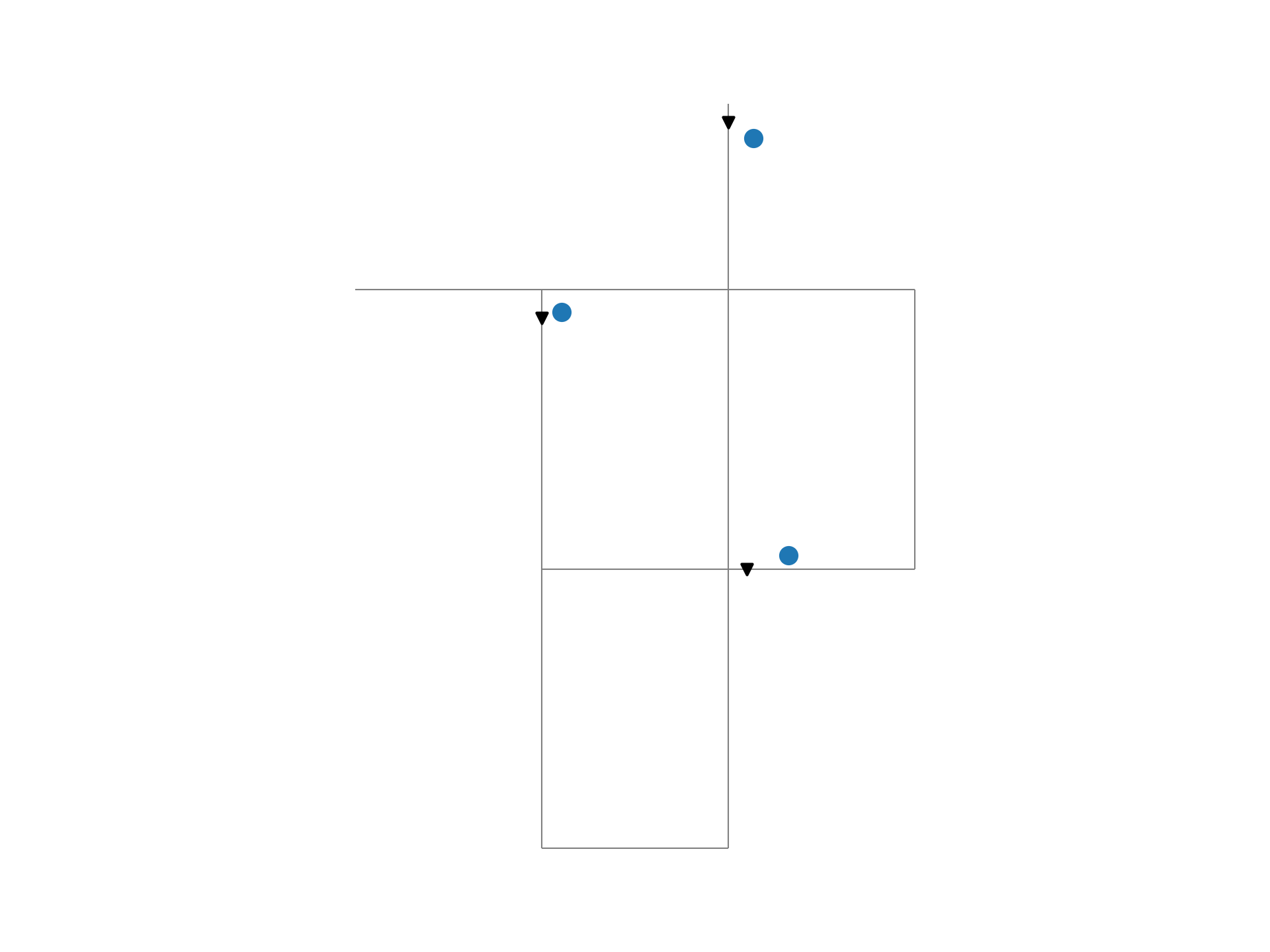
Figure 39 Net1 with example valve layer created by snapping points to lines, in which the blue circles are the isolation valve locations and the black triangles are the associated locations on the pipes.#
Find the intersect between geometries#
The intersect function is used to find the intersection between geometries.
This functionality can be used to identify faults, landslides, or other hazards that intersect pipes,
or assign community resilience indicators (e.g., population characteristics, economic), hazards/risks, or other data to network components.
When finding the intersection of GeoDataFrame A with GeoDataFrame B (where A and B can contain points, lines, or polygons), the function returns the following information (one entry for each geometry in A):
List of intersecting B geometry indices
Number of intersecting B geometries
The following additional information is returned when geometries in B are assigned a value:
List of intersecting B geometry values
Minimum B geometry value
Maximum B geometry value
Mean B geometry value
If A contains lines and B contains polygons, weighted mean value (weighted by intersecting length)
When the B geometry contains polygons, the user can optionally include the background in the intersection. This is useful when working with geometries that do not cover the entire region of interest. For example, while census tracts cover the entire region, hazard maps might contain gaps (regions with no hazard) that the user might want to include in the intersection.
The network file, Net1.inp, in EPSG:4326 CRS is used in the example below. Additional GIS data in the GeoJSON format is also in EPSG:4326 CRS. See Coordinate reference system for more information.
>>> wn = wntr.network.WaterNetworkModel('Net1')
>>> wn_gis = wntr.network.to_gis(wn, crs='EPSG:4326')
Assign earthquake probability to pipes#
GIS data that includes earthquake fault lines can be used in a resilience analysis to identify pipes which
have the potential to be damaged during an earthquake. The following example highlights the process to assign earthquake
probabilities to pipes. The example dataset of earthquake fault lines is a GeoDataFrame with a geometry column
that contains shapely.geometry.LineString geometries and a Pr column which contains probability of an earthquake over magnitude 7.
>>> earthquake_data = gpd.read_file('data/Net1_earthquake_data.geojson')
>>> print(earthquake_data)
     Pr                                geometry
0  0.50         LINESTRING (36 2, 44 44, 85 85)
1  0.75  LINESTRING (42 2, 45 27, 38 56, 30 85)
2  0.90         LINESTRING (40 2, 50 50, 60 85)
3  0.25  LINESTRING (30 2, 35 30, 40 50, 60 80)
The following example uses the function intersect to assign earthquake probability to pipes.
>>> pipe_Pr = wntr.gis.intersect(wn_gis.pipes, earthquake_data, 'Pr')
>>> print(pipe_Pr)
    intersections                  values  n   sum   min   max  mean
10             []                      []  0   NaN   NaN   NaN   NaN
11            [1]                  [0.75]  1  0.75  0.75  0.75  0.75
12      [0, 2, 3]        [0.5, 0.9, 0.25]  3  1.65  0.25  0.90  0.55
21   [0, 1, 2, 3]  [0.5, 0.75, 0.9, 0.25]  4  2.40  0.25  0.90  0.60
22             []                      []  0   NaN   NaN   NaN   NaN
31   [0, 1, 2, 3]  [0.5, 0.75, 0.9, 0.25]  4  2.40  0.25  0.90  0.60
110            []                      []  0   NaN   NaN   NaN   NaN
111            []                      []  0   NaN   NaN   NaN   NaN
112     [0, 2, 3]        [0.5, 0.9, 0.25]  3  1.65  0.25  0.90  0.55
113           [0]                   [0.5]  1  0.50  0.50  0.50  0.50
121            []                      []  0   NaN   NaN   NaN   NaN
122            []                      []  0   NaN   NaN   NaN   NaN
The data, water network model, and fault lines can be plotted as follows. The resulting Figure 40 illustrates Net1 with the intersection of pipes with the fault lines. The pipes are colored based upon their maximum earthquake probability.
>>> ax = earthquake_data.plot(column='Pr', alpha=0.5, cmap='bone', vmin=0, vmax=1)
>>> ax = wntr.graphics.plot_network(wn, link_attribute=pipe_Pr['max'], link_width=1.5,
...     node_range=[0,1], link_range=[0,1], ax=ax,
...     link_colorbar_label='Earthquake Probability')
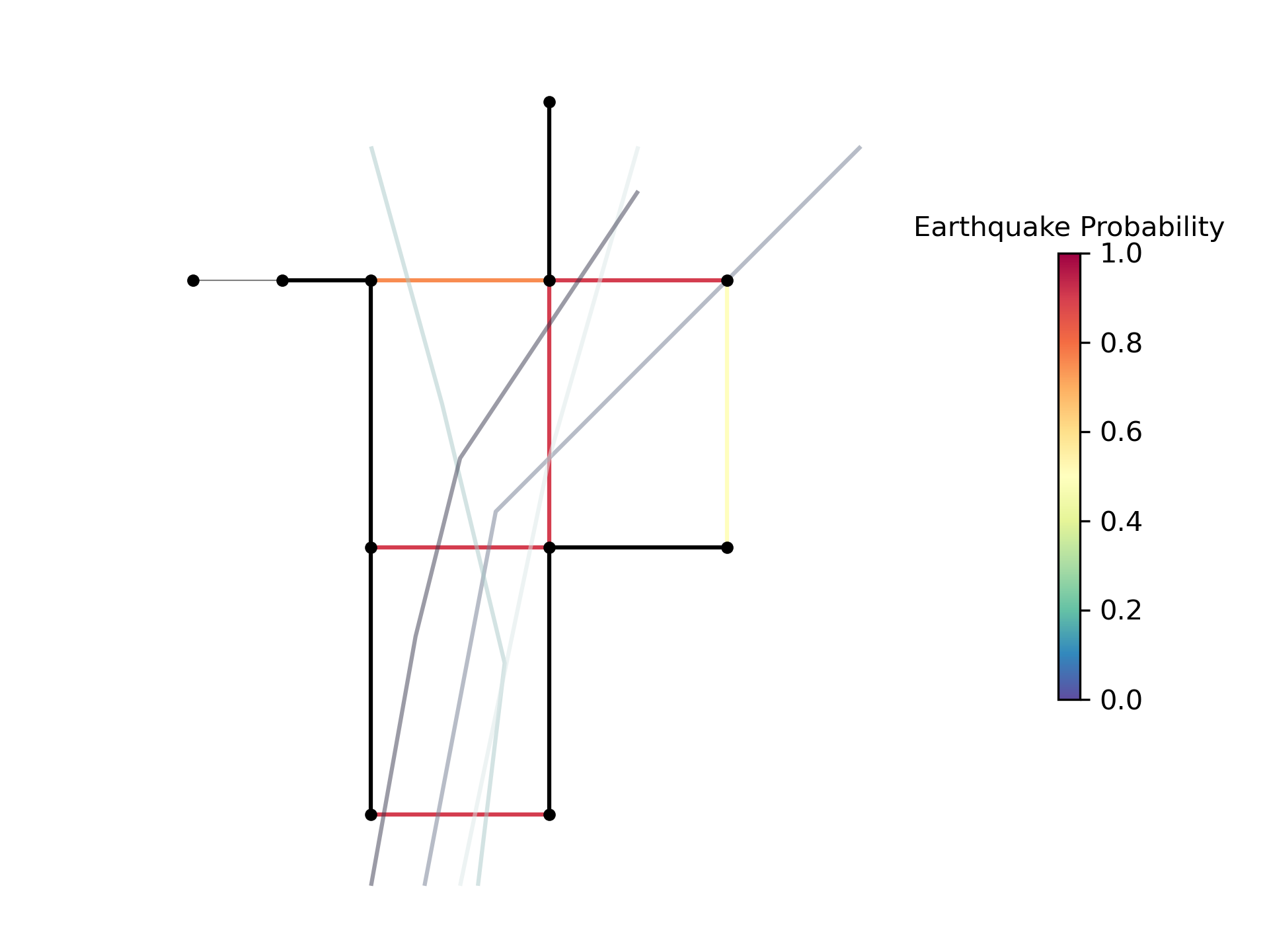
Figure 40 Net1 with example earthquake fault lines intersected with pipes, which are colored based upon their maximum earthquake probability.#
The intersect function can also be used to identify pipes that cross each fault simply by reversing the order in which the geometries intersect, as shown below:
>>> pipes_that_intersect_each_fault = wntr.gis.intersect(earthquake_data, wn_gis.pipes)
>>> print(pipes_that_intersect_each_fault)
            intersections  n
0  [112, 113, 12, 21, 31]  5
1            [11, 21, 31]  3
2       [112, 12, 21, 31]  4
3       [112, 12, 21, 31]  4
Assign landslide probability to pipes#
Landslide hazard zones GIS data can be used to identify pipes with the potential to be affected during a landslide.
The following example highlights the process to assign landslide probabilities to pipes. The landslide hazard zones example dataset
is a GeoDataFrame with a geometry column that contains shapely.geometry.LineString geometries and a
Pr column which contains the probability of damage from a landslide in that zone.
>>> landslide_data = gpd.read_file('data/Net1_landslide_data.geojson')
>>> print(landslide_data)
     Pr                                           geometry
0  0.50  POLYGON ((28.84615 22.23077, 28.7604 22.05079,...
1  0.75  POLYGON ((40.00708 1.83192, 33.00708 84.83192,...
2  0.90  POLYGON ((58.05971 44.48507, 58.11776 44.67615...
The following example uses the function intersect to assign landslide hazard zone probabilities to pipes.
This is very similar to the earthquake example above, except that the landslide hazards are polygons. Additionally, since the
hazard map does not include a “background” value that defines the probability of damage outside landslide zones,
the background conditions are included in the intersection function (i.e, the background value is assumed to be zero).
>>> pipe_Pr = wntr.gis.intersect(wn_gis.pipes, landslide_data, 'Pr',
...    include_background=True, background_value=0)
>>> print(pipe_Pr)
          intersections            values  n   sum  min   max   mean  weighted_mean
10         [BACKGROUND]             [0.0]  1  0.00  0.0  0.00  0.000          0.000
11      [BACKGROUND, 1]       [0.0, 0.75]  2  0.75  0.0  0.75  0.375          0.201
12         [BACKGROUND]             [0.0]  1  0.00  0.0  0.00  0.000          0.000
21   [BACKGROUND, 0, 1]  [0.0, 0.5, 0.75]  3  1.25  0.0  0.75  0.417          0.394
22      [BACKGROUND, 2]        [0.0, 0.9]  2  0.90  0.0  0.90  0.450          0.246
31      [BACKGROUND, 1]       [0.0, 0.75]  2  0.75  0.0  0.75  0.375          0.212
110        [BACKGROUND]             [0.0]  1  0.00  0.0  0.00  0.000          0.000
111     [BACKGROUND, 0]        [0.0, 0.5]  2  0.50  0.0  0.50  0.250          0.352
112        [BACKGROUND]             [0.0]  1  0.00  0.0  0.00  0.000          0.000
113        [BACKGROUND]             [0.0]  1  0.00  0.0  0.00  0.000          0.000
121     [BACKGROUND, 0]        [0.0, 0.5]  2  0.50  0.0  0.50  0.250          0.250
122        [BACKGROUND]             [0.0]  1  0.00  0.0  0.00  0.000          0.000
The data, water network model, and landslide zones can be plotted as follows. The resulting Figure 41 illustrates Net1 with the intersection of pipes with the landslide zones. The pipes are colored based upon their weighted mean landslide probability.
>>> ax = landslide_data.plot(column='Pr', alpha=0.5, cmap='bone', vmin=0, vmax=1)
>>> ax = wntr.graphics.plot_network(wn, link_attribute=pipe_Pr['weighted_mean'],
...     link_width=1.5, node_range=[0,1], link_range=[0,1], ax=ax,
...     link_colorbar_label='Landslide Probability')
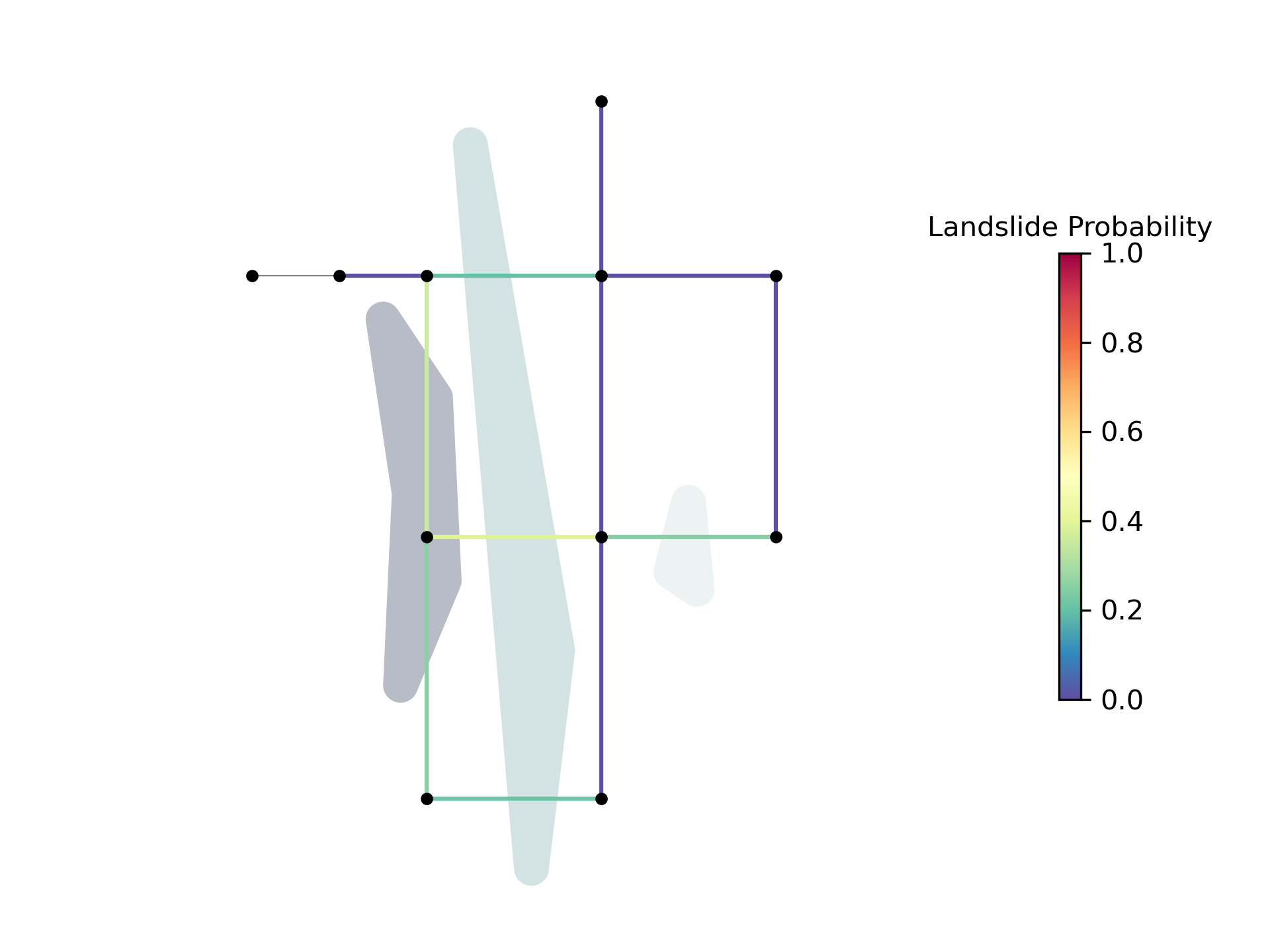
Figure 41 Net1 with example landslide zones intersected with pipes, which are colored based upon their weighted mean landslide probability.#
By reversing the order of GeoDataFrames in the intersection function, the pipes that intersect each landslide zone and information about the intersecting pipe diameters can also be identified:
>>> pipes_that_intersect_each_landslide = wntr.gis.intersect(landslide_data,
...     wn_gis.pipes, 'diameter')
>>> print(pipes_that_intersect_each_landslide)
    intersections                                             values  n    sum    min    max   mean
0  [111, 121, 21]                             [0.254, 0.2032, 0.254]  3  0.711  0.203  0.254  0.237
1    [11, 21, 31]  [0.35559999999999997, 0.254, 0.15239999999999998]  3  0.762  0.152  0.356  0.254
2            [22]                              [0.30479999999999996]  1  0.305  0.305  0.305  0.305
Assign demographic data to pipes and junctions#
GIS data that includes community resilience indicators (e.g., population characteristics, economic data),
hazards/risks, or other data can be used to identify
the effects of disasters to different portions of the community, which can help utilities to improve equitable resilience.
The following example highlights the process to assign demographic data to pipes and junctions. The demographic example dataset
is a GeoDataFrame with a geometry column that contains shapely.geometry.Polygon geometries along with
columns that store the mean income, the mean age, and the population within each census tract.
>>> demographic_data = gpd.read_file('data/Net1_demographic_data.geojson')
>>> print(demographic_data)
   mean_income  mean_age  population                                           geometry
0      63326.0      35.0      3362.0  POLYGON ((41.67813 82.75023, 41.98596 60.85779...
1      78245.0      31.0      5618.0  POLYGON ((23.21084 40.1916, 22.99063 27.71777,...
2      91452.0      40.0      5650.0  POLYGON ((22.99063 27.71777, 61.9372 16.36165,...
3      54040.0      39.0      5546.0  POLYGON ((61.9372 16.36165, 22.99063 27.71777,...
4      26135.0      38.0      5968.0  POLYGON ((61.9372 16.36165, 64.04456 22.10119,...
5      57620.0      31.0      4315.0  POLYGON ((44.48497 87.21487, 79.81144 71.92669...
6      44871.0      54.0      4547.0  POLYGON ((64.04456 22.10119, 51.72994 45.92347...
7      69067.0      55.0      2541.0  POLYGON ((46.01047 99.15725, 46.40654 99.33204...
The following example uses the function intersect
to assign the demographic data, specifically the mean income, to junctions and pipes.
>>> junction_demographics = wntr.gis.intersect(wn_gis.junctions, demographic_data,
...     'mean_income')
>>> print(junction_demographics)
   intersections     values  n      sum      min      max     mean
10           [0]  [63326.0]  1  63326.0  63326.0  63326.0  63326.0
11           [0]  [63326.0]  1  63326.0  63326.0  63326.0  63326.0
12           [5]  [57620.0]  1  57620.0  57620.0  57620.0  57620.0
13           [5]  [57620.0]  1  57620.0  57620.0  57620.0  57620.0
21           [3]  [54040.0]  1  54040.0  54040.0  54040.0  54040.0
22           [3]  [54040.0]  1  54040.0  54040.0  54040.0  54040.0
23           [6]  [44871.0]  1  44871.0  44871.0  44871.0  44871.0
31           [2]  [91452.0]  1  91452.0  91452.0  91452.0  91452.0
32           [2]  [91452.0]  1  91452.0  91452.0  91452.0  91452.0
>>> pipe_demographics = wntr.gis.intersect(wn_gis.pipes, demographic_data, 'mean_income')
>>> print(pipe_demographics)
    intersections              values  n       sum      min      max     mean  weighted_mean
10            [0]           [63326.0]  1   63326.0  63326.0  63326.0  63326.0      63326.000
11         [0, 5]  [63326.0, 57620.0]  2  120946.0  57620.0  63326.0  60473.0      61002.920
12            [5]           [57620.0]  1   57620.0  57620.0  57620.0  57620.0      57620.000
21            [3]           [54040.0]  1   54040.0  54040.0  54040.0  54040.0      54040.000
22         [3, 6]  [54040.0, 44871.0]  2   98911.0  44871.0  54040.0  49455.5      47067.895
31            [2]           [91452.0]  1   91452.0  91452.0  91452.0  91452.0      91452.000
110        [5, 7]  [57620.0, 69067.0]  2  126687.0  57620.0  69067.0  63343.5      60580.117
111        [0, 3]  [63326.0, 54040.0]  2  117366.0  54040.0  63326.0  58683.0      60953.558
112        [3, 5]  [54040.0, 57620.0]  2  111660.0  54040.0  57620.0  55830.0      56596.728
113        [5, 6]  [57620.0, 44871.0]  2  102491.0  44871.0  57620.0  51245.5      53707.370
121        [2, 3]  [91452.0, 54040.0]  2  145492.0  54040.0  91452.0  72746.0      73586.482
122        [2, 3]  [91452.0, 54040.0]  2  145492.0  54040.0  91452.0  72746.0      66314.037
The data, water network model, and census tracts can be plotted as follows. The resulting Figure 42 illustrates Net1 with the intersection of junctions and pipes with the census tracts (polygons). The junctions and pipes are colored with their mean income and weighted mean income, respectively. Note that the color scale for the census tracts (polygons) is different than the junction and pipe attributes.
>>> ax = demographic_data.plot(column='mean_income', alpha=0.5,
...     cmap='bone', vmin=10000, vmax=100000)
>>> ax = wntr.graphics.plot_network(wn, node_attribute=junction_demographics['mean'],
...     link_attribute=pipe_demographics['weighted_mean'], link_width=1.5,
...     node_range=[40000,80000], link_range=[40000,80000], ax=ax)
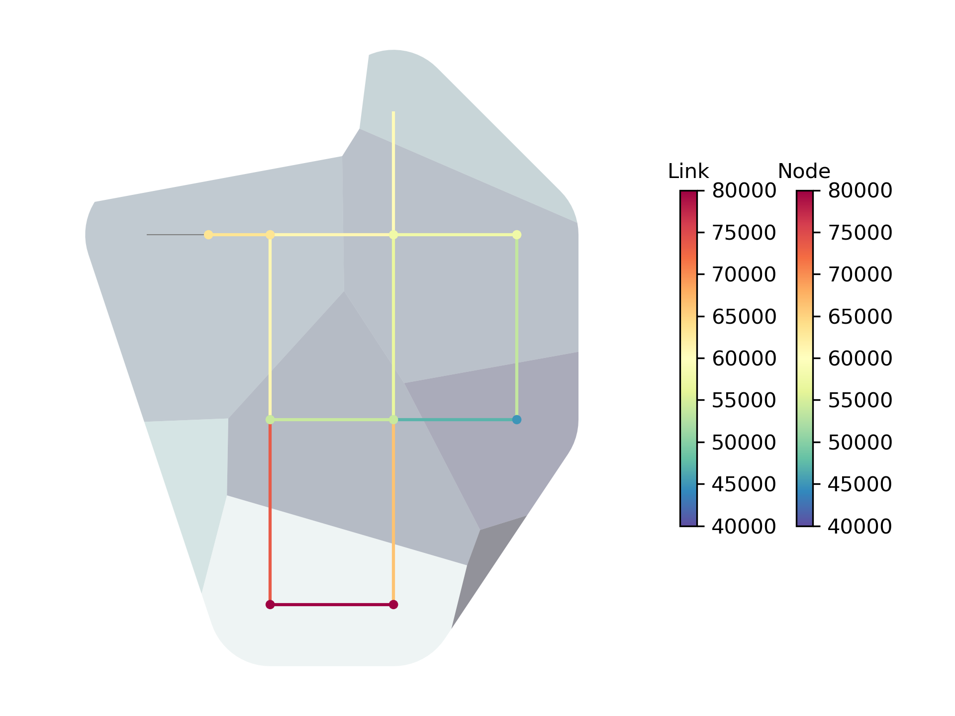
Figure 42 Net1 with mean income demographic data intersected with junctions and pipes.#
Sample raster at points geometries#
The sample_raster function can be used to sample a raster file at point geometries,
such as the nodes of a water network. A common use case for this function is to assign elevation to the
nodes of a water network model, however other geospatial information such as hazard data could be sampled
using this function.
The network file, Net1.inp, in EPSG:4326 CRS is used in the example below. The raster data in the GeoTIFF format is also in EPSG:4326 CRS. See Coordinate reference system for more information.
>>> wn = wntr.network.WaterNetworkModel('Net1')
>>> wn_gis = wntr.network.to_gis(wn, crs='EPSG:4326')
Sample elevations at junctions#
Elevation is an essential attribute for accurate simulation of pressure in a water network and is commonly provided in GeoTIFF (.tif) files. The following example shows how such files can be sampled and assigned to the junctions and tanks of a network. Note that elevation data generally needs to be adjusted to account for buried pipes.
>>> elevation_data_path = 'data/Net1_elevation_data.tif'
>>> junctions = wn_gis.junctions
>>> junction_elevations = wntr.gis.sample_raster(junctions, elevation_data_path)
>>> print(junction_elevations)
name
10    1400.0
11    2100.0
12    3500.0
13    4900.0
21    1200.0
22    2000.0
23    2800.0
31     300.0
32     500.0
dtype: float64
>>> tanks = wn_gis.tanks
>>> tank_elevations = wntr.gis.sample_raster(tanks, elevation_data_path)
>>> print(tank_elevations)
name
2    4500.0
dtype: float64
To use these elevations for hydraulic simulations, they need to be added to the water network object.
>>> for junction_name in wn.junction_name_list:
...     junction = wn.get_node(junction_name)
...     junction.elevation = junction_elevations[junction_name]
>>> for tank_name in wn.tank_name_list:
...     tank = wn.get_node(tank_name)
...     tank.elevation = tank_elevations[tank_name]
The sampled elevations can be plotted as follows. The resulting Figure 43 illustrates Net1 with the elevations sampled from the raster file.
>>> ax = wntr.graphics.plot_network(wn, node_attribute="elevation", link_width=1.5,
...     node_size=40, node_colorbar_label='Raster Elevation')
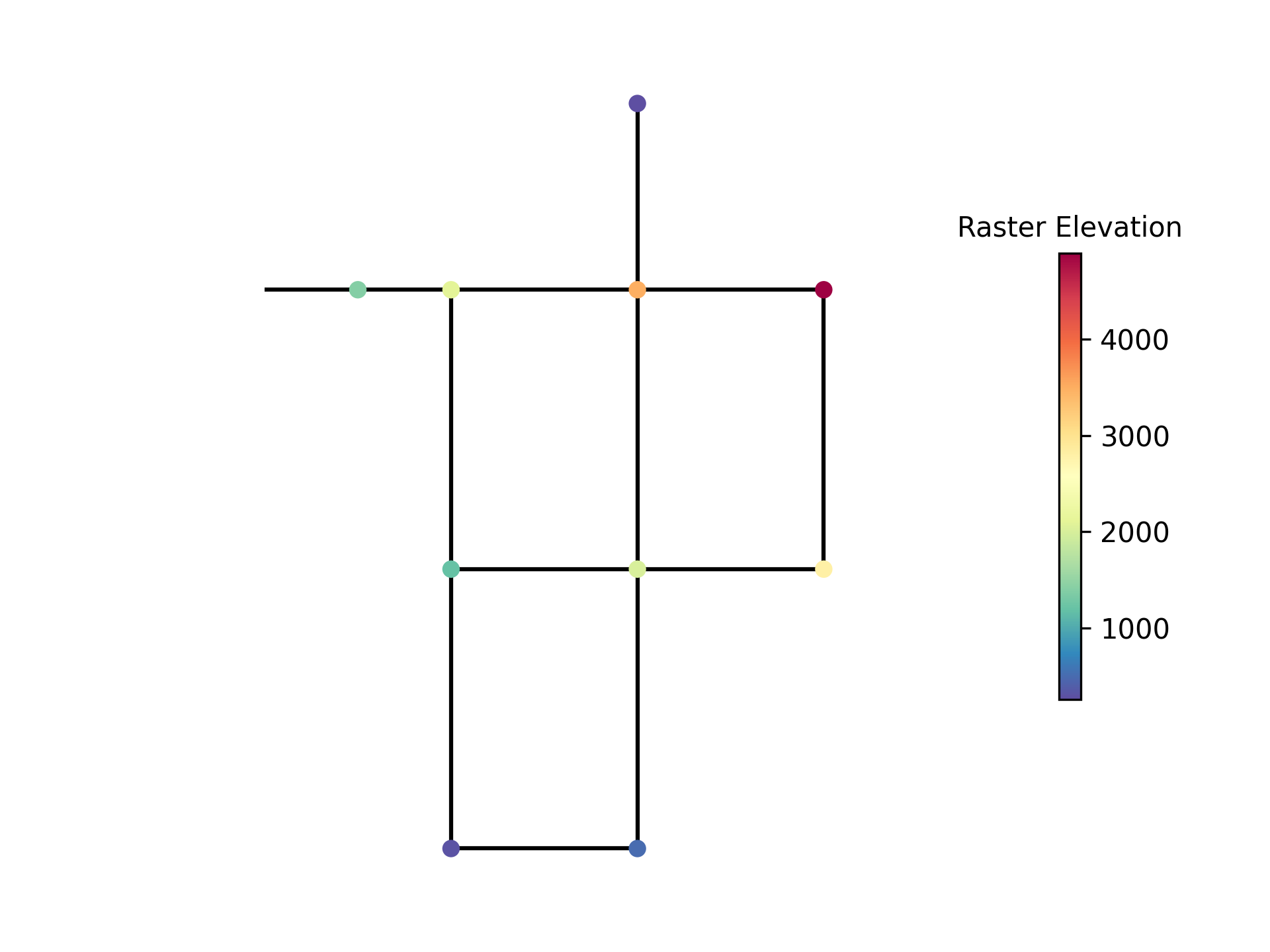
Figure 43 Net1 with elevations sampled from raster.#
Connect lines#
The connect_lines function can be used connect line geometries that do not connect.
This is useful, for example, when utility pipe data does not perfectly connect at line endpoints and junction coordinates are unknown.
The connect_lines function takes a GeoDataFrame with LineString geometries and a distance threshold and returns
a line GeoDataFrame with connected LineStrings and
a node GeoDataFrame with Point coordinates.
Connect pipe data#
A WaterNetworkModel requires pipe data with start_node_name and end_node_name attributes.
These node names refer to Junctions, Tanks, or Reservoirs.
When this connectivity information is not known (i.e., the pipe data has no start_node_name and end_node_name), the
connect_lines function can be used to connect line end points with a user specified distance threshold.
The following example creates disconnected pipe data using Net1, and then generates the data needed to create a connected WaterNetworkModel. This assumes that all start and end nodes are Junctions.
>>> wn = wntr.network.WaterNetworkModel('Net1')
>>> wn_gis = wntr.network.to_gis(wn, crs='EPSG:2236')
>>> original_pipes = wn_gis.pipes
To create the disconnected pipe data in this example, the original pipes were rotated (+/- 5 degrees) and scaled (90% in the x and y direction). The disconnected pipe data is missing start and end node names, and end points do not connect.
Connect the disconnected pipes using a distance threshold of 5 ft (same distance units as the CRS)
>>> distance_threshold = 5 # ft
>>> pipes, junctions = wntr.gis.connect_lines(disconnected_pipes, distance_threshold)
Figure 44 illustrates the original pipe data, the disconnected pipe data, and the connected pipe and junction data.
>>> ax = disconnected_pipes.plot(ax=ax, color='r', label='Disconnected pipe data')
>>> ax = pipes.plot(ax=ax, color='k', linewidth=6, alpha=0.35, label='Connected pipe data')
>>> ax = junctions.plot(ax=ax, color='k', label='Connected junctions')
>>> legend = ax.legend()
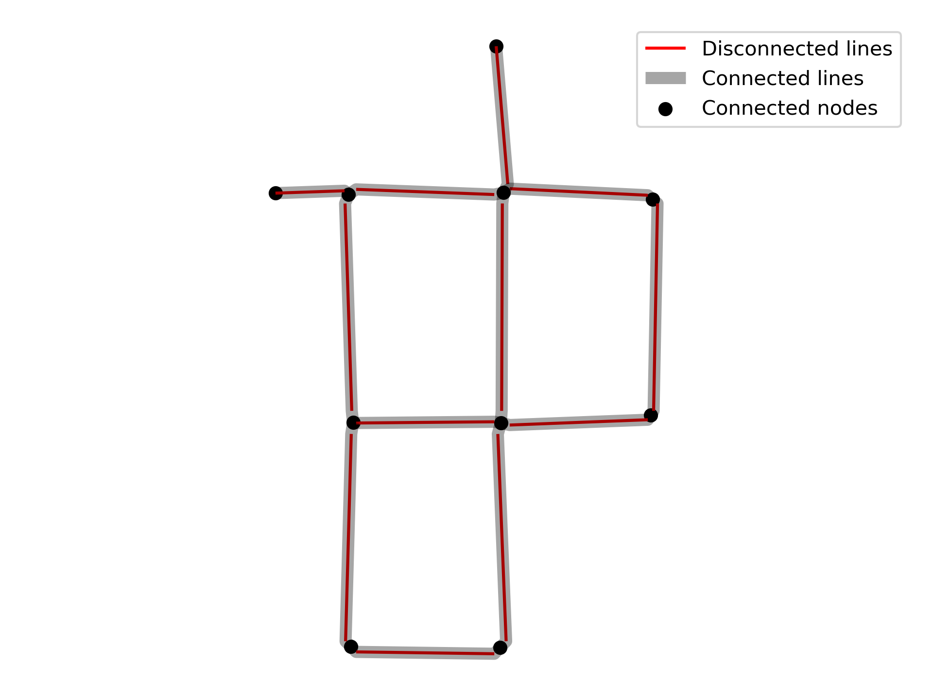
Figure 44 Connected pipes and junctions from a disconnected dataset#
Use the junction and pipe data to create a basic WaterNetworkModel (without tanks, reservoirs, pumps, or valves).
>>> gis_data = wntr.gis.WaterNetworkGIS({"junctions": junctions, "pipes": pipes})
>>> wn = wntr.network.from_gis(gis_data)