Hydraulic simulation#
WNTR contains two simulators: the EpanetSimulator and the WNTRSimulator. See Software framework and limitations for more information on features and limitations of these simulators.
EpanetSimulator#
The EpanetSimulator can be used to run EPANET 2.00.12 Programmer’s Toolkit [24] or EPANET 2.2.0 Programmer’s Toolkit [23]. EPANET 2.2.0 is used by default and runs demand-driven and pressure dependent hydraulic analysis. EPANET 2.00.12 runs demand-driven hydraulic analysis only. Both versions can also run water quality simulations, as described in Water quality simulation.
The user can switch between pressure dependent demand (PDD) or demand-driven (DD) hydraulic simulation by setting
the wn.options.hydraulic.demand_model option.
.. doctest:
>>> import wntr

>>> wn = wntr.network.WaterNetworkModel('Net3')
>>> wn.options.hydraulic.demand_model = 'DD'
>>> wn.options.hydraulic.demand_model = 'PDD'
Note
EPANET 2.2.0 uses the terms demand-driven analysis (DDA) and pressure driven analysis (PDA). In WNTR, the user can select demand-driven using ‘DD’ or ‘DDA’ and pressure dependent demand using ‘PDD’ or ‘PDA’.
A hydraulic simulation using the EpanetSimulator is run using the following code:
>>> sim = wntr.sim.EpanetSimulator(wn)
>>> results = sim.run_sim() # by default, this runs EPANET 2.2.0
The user can switch between EPANET version 2.00.12 and 2.2.0 as shown below:
>>> results1 = sim.run_sim(version=2.0) # runs EPANET 2.00.12
>>> results2 = sim.run_sim(version=2.2) # runs EPANET 2.2.0
WNTRSimulator#
The WNTRSimulator is a hydraulic simulation engine based on the same equations as EPANET. The WNTRSimulator does not include equations to run water quality simulations. The WNTRSimulator includes the option to simulate leaks, and run hydraulic simulations in demand-driven or pressure dependent demand mode.
As with the EpanetSimulator, the user can switch between DD and PDD by setting
the wn.options.hydraulic.demand_model option.
>>> wn.options.hydraulic.demand_model = 'DD'
>>> wn.options.hydraulic.demand_model = 'PDD'
A hydraulic simulation using the WNTRSimulator is run using the following code:
>>> sim = wntr.sim.WNTRSimulator(wn)
>>> results = sim.run_sim()
More information on the simulators can be found in the API documentation, under
EpanetSimulator and
WNTRSimulator.
The simulators use different solvers for the system of hydraulic equations; as such, small differences in the results
are expected.
While the EpanetSimulator uses Todini’s Global Gradient Algorithm to solve the system of equations,
the WNTRSimulator uses a Newton-Raphson algorithm.
Hydraulic options#
The hydraulic simulation options include headloss model, viscosity, diffusivity, trails, accuracy, default pattern, demand multiplier, demand model, minimum pressure, required pressure, and pressure exponent. Note that EPANET 2.00.12 does not use the demand model, minimum pressure, required pressure, or pressure exponent. Options that directly apply to hydraulic simulation that are not used in the WNTRSimulator are described in Limitations.
When creating a water network model from an EPANET INP file, hydraulic options are populated from the [OPTIONS] sections of the EPANET INP file. All of these options can be modified in WNTR and then written to an EPANET INP file. More information on water network options can be found in Options.
Mass balance at nodes#
Both simulators use the mass balance equations from EPANET [24]:
where \(P_{n}\) is the set of pipes connected to node \(n\), \(q_{p,n}\) is the flow rate of water into node \(n\) from pipe \(p\) (m³/s), \(D_{n}^{act}\) is the actual demand out of node \(n\) (m³/s), and \(N\) is the set of all nodes. If water is flowing out of node \(n\) and into pipe \(p\), then \(q_{p,n}\) is negative. Otherwise, it is positive.
Headloss in pipes#
Both simulators use conservation of energy formulas from EPANET [24]. While the EpanetSimulator can use the Hazen-Williams and Chezy-Manning pipe head loss formulas, the WNTRSimulator uses only the Hazen-Williams head loss formula, shown below.
where \(h_{L}\) is the headloss in the pipe (m), \(C\) is the Hazen-Williams roughness coefficient (unitless), \(d\) is the pipe diameter (m), \(L\) is the pipe length (m), \(q\) is the flow rate of water in the pipe (m³/s), \(H_{n_{j}}\) is the head at the starting node (m), and \(H_{n_{i}}\) is the head at the ending node (m).
The flow rate in a pipe is positive if water is flowing from the starting node to the ending node and negative if water is flowing from the ending node to the starting node.
The Hazen-Williams headloss formula is not valid for negative flow rates. Therefore, the WNTRSimulator uses a reformulation of this constraint.
For \(q<0\):
For \(q \geq 0\):
These equations are symmetric across the origin and valid for any \(q\). Thus, this equation can be used for flow in either direction. However, the derivative with respect to \(q\) at \(q = 0\) is \(0\). In certain scenarios, this can cause the Jacobian matrix of the set of hydraulic equations to become singular (when \(q=0\)). To overcome this limitation, the WNTRSimulator splits the domain of \(q\) into segments to create a piecewise smooth function.
See EPANET documentation for more details on analysis algorithms used by EPANET (and therefore used by the EpanetSimulator).
Demand-driven simulation#
In a demand-driven simulation, the pressure in the system depends on the node demands. The mass balance and headloss equations described above are solved assuming that node demands are known and satisfied. This assumption is reasonable under normal operating conditions and for use in network design. Both simulators can run hydraulics using demand-driven simulation.
Pressure dependent demand simulation#
In situations that lead to low pressure conditions (i.e., fire fighting, power outages, pipe leaks), consumers do not always receive their requested demand and a pressure dependent demand simulation is recommended. In a pressure dependent demand simulation, the delivered demand depends on the pressure. The mass balance and headloss equations described above are solved by simultaneously determining demand along with the network pressures and flow rates.
Both simulators can run hydraulics using a pressure dependent demand simulation according to the following pressure-demand relationship [33]:
where \(d\) is the actual demand (m³/s), \(D_f\) is the desired demand (m³/s), \(p\) is the pressure (Pa), \(P_f\) is the required pressure (Pa) - this is the pressure above which the consumer should receive the desired demand, and \(P_0\) is the minimum pressure (Pa) - this is the pressure below which the consumer cannot receive any water, \(1/e\) is the pressure exponent, usually set equal to 0.5.
Figure 12 illustrates the pressure-demand relationship using both the demand-driven and pressure dependent demand simulations. In the example, \(D_f\) is 0.0025 m³/s (39.6 GPM), \(P_f\) is 30 psi (21.097 m), and \(P_0\) is 5 psi (3.516 m). Using the demand-driven simulation, the demand is equal to \(D_f\) regardless of pressure. Using the pressure dependent demand simulation, the demand starts to decrease when the pressure is below \(P_f\) and goes to 0 when pressure is below \(P_0\).
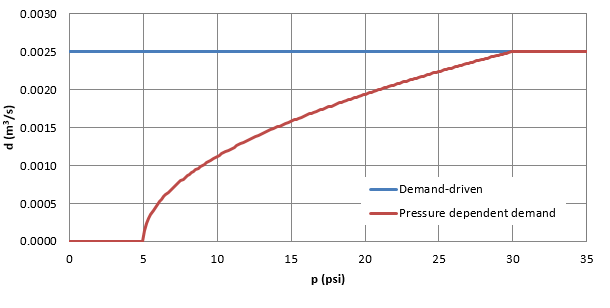
Figure 12 Relationship between pressure (p) and demand (d) using both the demand-driven and pressure dependent demand simulations.#
The required pressure, minimum pressure, and pressure exponent are defined in the global hydraulic options, and can be reset as shown in the following example.
>>> wn.options.hydraulic.required_pressure = 21.097 # 30 psi = 21.097 m
>>> wn.options.hydraulic.minimum_pressure  = 3.516 # 5 psi = 3.516 m
>>> wn.options.hydraulic.pressure_exponent = 0.55
Note
The default values for required pressure, minimum pressure and pressure exponent are 0.07 m (0.1 psi), 0 m (0 psi), and 0.5, respectively. This matches EPANET specifications. If the user does not increase the default required pressure value, then a PDD simulation will be very similar to a DD simulation. WNTR also enforces 0.07 m (0.1 psi) as the lowest value for required pressure to match EPANET specifications.
When using the WNTRSimulator, the required pressure, minimum pressure, and pressure exponent can vary throughout the network. By default, each junction’s required pressure, minimum pressure, and pressure exponent is set to None and the global value is used in the hydraulic options to define the PDD constraint for that junction. If the user defines required pressure, minimum pressure, or pressure exponent on a junction, those values will override the required pressure, minimum pressure, and pressure exponent defined in the global hydraulic options when defining the PDD constraint for that junction. The following example defines required pressure, minimum pressure, and pressure exponent on junction 121.
>>> junction = wn.get_node('121')
>>> junction.required_pressure = 14.065 # 20 psi = 14.065 m
>>> junction.minimum_pressure = 0.352 # 0.5 psi = 0.352 m
>>> junction.pressure_exponent = 0.4
The ability to use spatially variable required pressure, minimum pressure, and pressure exponent is only available when using the WNTRSimulator. The EpanetSimulator always uses the global values in the hydraulic options.
Leak model#
The WNTRSimulator includes the ability to add leaks to the network using a leak model. As such, emitter coefficients defined in the water network model options are not used by the WNTRSimulator. Users interested in using the EpanetSimulator to model leaks can still do so by defining emitter coefficients.
When using the WNTRSimulator, leaks are modeled with a general form of the equation proposed by Crowl and Louvar [6] where the mass flow rate of fluid through the hole is expressed as:
where \(d_{leak}\) is the leak demand (m³/s), \(C_d\) is the discharge coefficient (unitless), \(A\) is the area of the hole (m²), \(\alpha\) is an exponent related to characteristics of the leak (unitless), \(p\) is the gauge pressure (Pa), \(h\) is the gauge head (m), \(g\) is the acceleration of gravity (m/s²), and \(\rho\) is the density of the fluid (kg/m³).
The default discharge coefficient is 0.75 (assuming turbulent flow) [17], but the user can specify other values if needed. The value of \(\alpha\) is set to 0.5 (assuming large leaks out of steel pipes) [17] and currently cannot be changed by the user.
Leaks can be added to junctions and tanks. A pipe break is modeled using a leak area large enough to drain the pipe. WNTR includes methods to add leaks to any location along a pipe by splitting the pipe into two sections and adding a node.
Figure 13 illustrates leak demand. In the example, the diameter of the leak is set to 0.5 cm, 1.0 cm, and 1.5 cm.
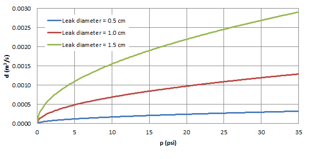
Figure 13 Relationship between leak demand (d) and pressure (p).#
The following example adds a leak to the water network model.
>>> node = wn.get_node('123')
>>> node.add_leak(wn, area=0.05, start_time=2*3600, end_time=12*3600)
Pause and restart#
The WNTRSimulator includes the ability to:
Reset initial values and re-simulate using the same water network model. Initial values include simulation time, tank head, reservoir head, pipe status, pump status, and valve status.
Pause a hydraulic simulation, change network operations, and then restart the simulation.
Save the water network model and results to files and reload for future analysis.
These features are helpful when evaluating various response action plans or when simulating long periods of time where the time resolution might vary.
The following example runs a hydraulic simulation for 10 hours and then restarts the simulation for another 14 hours. The results from the first 10 hours and last 14 hours can be combined for analysis or analyzed separately. Furthermore, network operations can be modified between simulations.
>>> wn.options.time.duration = 10*3600
>>> sim = wntr.sim.WNTRSimulator(wn)
>>> first_10_hours_results = sim.run_sim()
>>> wn.options.time.duration = 24*3600
>>> sim = wntr.sim.WNTRSimulator(wn)
>>> last_14_hours_results = sim.run_sim()
To restart the simulation from time zero, the user has several options.
Use the existing water network model and reset initial conditions. Initial conditions include simulation time, tank head, reservoir head, pipe status, pump status, and valve status. This option is useful when only initial conditions have changed between simulations.
>>> wn.reset_initial_values()
Save the water network model to a file and reload that file each time a simulation is run. A pickle file is generally used for this purpose. A pickle file is a binary file used to serialize and de-serialize a Python object. More information on the use of pickle files can be found at https://docs.python.org/3/library/pickle.html. This option is useful when the water network model contains custom controls that would not be reset using the option 1, or when the user wants to change operations between simulations.
The following example saves the water network model to a file before using it in a simulation.
>>> import pickle

>>> f=open('wn.pickle','wb')
>>> pickle.dump(wn,f)
>>> f.close()
>>> sim = wntr.sim.WNTRSimulator(wn)
>>> results = sim.run_sim()
The next example reload the water network model from the file before the next simulation.
>>> f=open('wn.pickle','rb')
>>> wn = pickle.load(f)
>>> f.close()
>>> sim = wntr.sim.WNTRSimulator(wn)
>>> results = sim.run_sim()
If these options do not cover user specific needs, then the water network model would need to be recreated between simulations or reset manually by changing individual attributes to the desired values. Note that when using the EpanetSimulator, the model is reset each time it is used in a simulation.