Resilience metrics

Resilience of water distribution systems refers to the design, maintenance, and operations of that system. All these aspects must work together to limit the effects of disasters and enable rapid return to normal delivery of safe water to customers. Numerous resilience metrics have been suggested [26]. These metrics generally fall into five categories: topographic, hydraulic, water quality, water security, and economic [26]. When quantifying resilience, it is important to understand which metric best defines resilience for a particular scenario. WNTR includes many metrics to help users compare resilience using different methods.

The following sections outline metrics that can be computed using WNTR, including:

• Topographic metrics (Table 6)

• Hydraulic metrics (Table 7)

• Water quality metrics (Table 8)

• Water security metrics (Table 9)

• Economic metrics (Table 10)

While some metrics define resilience as a single system-wide quantity, other metrics define quantities that are a function of time, space, or both. For this reason, state transition plots [3] and network graphics are useful ways to visualize resilience and compare metrics, as shown in Figure 15. In the state transition plot, the x-axis represents time (before, during, and after a disruptive incident). The y-axis represents performance. This can be any time varying resilience metric that responds to the disruptive state. State transition plots are often generated to show time varying performance of the system, but they can also represent the time varying performance of individual components, like tanks or pipes. Network graphics are useful to visualize resilience metrics that vary with respect to location. For metrics that vary with respect to time and space, network animation can be used to illustrate resilience.

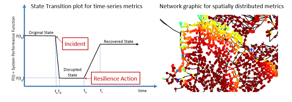
Figure 15 Example state transition plot (left) and network graphic (right) used to visualize resilience.

Topographic metrics

Topographic metrics, based on graph theory, can be used to assess the connectivity of water distribution networks. These metrics rely on the physical layout of the network components and can be used to understand how the underlying structure and connectivity constrains resilience. For example, a regular lattice, where each node has the same number of edges (except at the border), is considered to be the most reliable graph structure. On the other hand, a random lattice has nodes and edges that are placed according to a random process. A real world water distribution system probably lies somewhere in between a regular lattice and a random lattice in terms of structure and reliability.

Commonly used topographic metrics are listed in Table 6. Many of these metrics can be computed using NetworkX directly (see https://networkx.github.io/ for more information). WNTR includes additional topographic metrics to help compute resilience.

Table 6 Topographic Resilience Metrics

Metric	Description
Node degree and terminal nodes	Node degree is the number of links adjacent to a node. Node degree is a measure of the number of branches in a network. A node with degree 0 is not connected to the network. Terminal nodes have degree 1. A node connected to every node (including itself) has a degree equal to the number of nodes in the network. The average node degree is a system-wide metric used to describe the number of connected links in a network.
Link density	Link density is the ratio between the total number of links and the maximum number of links in the network. If links are allowed to connect a node to itself, then the maximum number of links is \({n}^{2}\), where \(n\) is the number of nodes. Otherwise, the maximum number of nodes is \(n(n-1)\). Link density is 0 for a graph without edges and 1 for a dense graph. The density of multigraphs can be higher than 1.
Eccentricity and diameter	Eccentricity is the maximum number of links between a node and all other nodes in the graph. Eccentricity is a value between 0 and the number of links in the network. Diameter is the maximum eccentricity in the network. Eccentricity and diameter can only be computed using undirected, connected networks.
Betweenness centrality	Betweenness centrality is the fraction of shortest paths that pass through each node. Betweenness coefficient is a value between 0 and 1. Central point dominance is the average difference in betweenness centrality of the most central point (having the maximum betweenness centrality) and all other nodes.
Closeness centrality	Closeness centrality is the inverse of the sum of shortest path from one node to all other nodes.
Articulation points	A node is considered an articulation point if the removal of that node (along with all its incident edges) increases the number of connected components of a network. Density of articulation points is the ratio of the number of articulation points and the total number of nodes. Density of articulation points is a value between 0 and 1.
Bridges	A link is considered a bridge if the removal of that link increases the number of connected components in the network. The ratio of the number of bridges and the total number of links in the network is the bridge density. Bridge density is a value between 0 and 1.
Simple paths	A simple path is a path between two nodes that does not repeat any nodes. Paths can be time dependent, if related to flow direction.
Shortest path lengths	Shortest path lengths is the minimum number of links between a source node and all other nodes in the network. Shortest path length is a value between 0 and the number of links in the network. The average shortest path length is a system-wide metric used to describe the number of links between a node and all other nodes.
Valve segmentation	Valve segmentation groups links and nodes into segments based on the location of isolation valves. Valve segmentation returns a segment number for each node and link, along with the number of nodes and links in each segment.
Valve segment attributes	Valve segment attributes include the number of valves surrounding each valve and (optionally) the increase in segment demand if a given valve is removed, and the increase in segment pipe length if a given valve is removed. The increase in segment demand is expressed as a fraction of the max segment demand associated with that valve. Likewise, the increase in segment pipe length is expressed as a fraction of the max segment pipe length associated with that valve.

To compute topographic metrics, a NetworkX MultiDiGraph is first extracted from a WaterNetworkModel. Note that some metrics require an undirected graph or a graph with a single edge between two nodes.

>>> import networkx as nx
>>> import wntr 

>>> wn = wntr.network.WaterNetworkModel('networks/Net3.inp') 
>>> G = wn.to_graph() # directed multigraph
>>> uG = G.to_undirected() # undirected multigraph
>>> sG = nx.Graph(uG) # undirected simple graph (single edge between two nodes)

The following examples compute topographic metrics. Note that many of these metrics use NetworkX directly, while others use metrics included in WNTR.

• Node degree and terminal nodes

  >>> node_degree = G.degree()
  >>> terminal_nodes = wntr.metrics.terminal_nodes(G)
  

• Link density

  >>> link_density = nx.density(G)
  

• Diameter and eccentricity

  >>> diameter = nx.diameter(uG)
  >>> eccentricity = nx.eccentricity(uG)
  

• Betweenness centrality and central point dominance

  >>> betweenness_centrality = nx.betweenness_centrality(sG)
  >>> central_point_dominance = wntr.metrics.central_point_dominance(G)
  

• Closeness centrality

  >>> closeness_centrality = nx.closeness_centrality(G)
  

• Articulation points and bridges

  >>> articulation_points = list(nx.articulation_points(uG))
  >>> bridges = wntr.metrics.bridges(G)
  

• Shortest path lengths between all nodes and average shortest path length

  >>> shortest_path_length = nx.shortest_path_length(uG)
  >>> ave_shortest_path_length = nx.average_shortest_path_length(uG)
  

• Paths between two nodes in a weighted graph, where the graph is weighted by flow direction from a hydraulic simulation

  >>> sim = wntr.sim.EpanetSimulator(wn)
  >>> results = sim.run_sim()
  
  >>> flowrate = results.link['flowrate'].iloc[-1,:] # flowrate from the last timestep
  >>> G = wn.to_graph(link_weight=flowrate, modify_direction=True)
  >>> all_paths = nx.all_simple_paths(G, '119', '193')
  

• Valve segmentation, where each valve is defined by a node and link pair (see Valve layer)

  >>> valve_layer = wntr.network.generate_valve_layer(wn, 'random', 40)
  >>> node_segments, link_segments, segment_size = wntr.metrics.valve_segments(G,
  ...     valve_layer)
  

• Valve segment attributes

  >>> average_expected_demand = wntr.metrics.average_expected_demand(wn)
  >>> link_lengths = wn.query_link_attribute('length')
  >>> valve_attributes = wntr.metrics.valve_segment_attributes(valve_layer,
  ...     node_segments, link_segments, average_expected_demand, link_lengths)
  

Hydraulic metrics

Hydraulic metrics are based on flow, demand, and/or pressure. With the exception of expected demand and average expected demand, the calculation of these metrics requires simulation of network hydraulics that reflect how the system operates under normal or abnormal conditions. Hydraulic metrics included in WNTR are listed in Table 7.

Table 7 Hydraulic Resilience Metrics

Metric	Description
Pressure	To determine the number of node-time pairs above or below a specified pressure threshold, use the query method on results.node[‘pressure’].
Demand	To determine the number of node-time pairs above or below a specified demand threshold, use the query method on results.node[‘demand’]. This method can be used to compute the fraction of delivered demand, from [18].
Water service availability	Water service availability is the ratio of delivered demand to the expected demand. This metric can be computed as a function of time or space using the water_service_availability method. This method can be used to compute the fraction of delivered volume, from [18].
Todini index	The Todini index [25] is related to the capability of a system to overcome failures while still meeting demands and pressures at nodes. The Todini index defines resilience at a specific time as a measure of surplus power at each node. The Todini index can be computed using the todini_index method.
Modified resilience index	The modified resilience index [11] is similar to the Todini index, but is only computed at junctions. The metric defines resilience at a specific time as a measure of surplus power at each junction or as a system average. The modified resilience index can be computed using the modified_resilience_index method.
Tank capacity	Tank capacity is the ratio of current water volume stored in tanks to the maximum volume of water that can be stored. This metric is measured at each tank as a function of time and ranges between 0 and 1. A value of 1 indicates that tank storage is maximized, while a value of 0 means there is no water stored in the tank. Tank capacity can be computed using the tank_capacity method.
Entropy	Entropy [2] is a measure of uncertainty in a random variable. In a water distribution network model, the random variable is flow in the pipes and entropy can be used to measure alternate flow paths when a network component fails. A network that carries maximum entropy flow is considered reliable with multiple alternate paths. Connectivity will change at each timestep, depending on the flow direction. The to_graph method can be used to generate a weighted graph. Entropy can be computed using the entropy method.
Expected demand	Expected demand is computed at each node and timestep based on node demand, demand pattern, and demand multiplier [27]. The metric can be computed using the expected_demand method. This method does not require running a hydraulic simulation.
Average expected demand	Average expected demand per day is computed at each node based on node demand, demand pattern, and demand multiplier [27]. The metric can be computed using the average_expected_demand method. This method does not require running a hydraulic simulation.
Population impacted	Population that is impacted by a specific quantity can be computed using the population_impacted method. For example, this method can be used to compute the population impacted by pressure below a specified threshold. Population per node is computed using the method population, which divides the average expected demand by the average volume of water consumed per capita per day. The default value for average volume of water consumed per capita per day is 200 gallons/day and can be modified by the user.

The following examples compute hydraulic metrics, including:

• Nodes and times when pressure exceeds a threshold, using results from a hydraulic simulation

  >>> import numpy as np
  
  >>> wn.options.hydraulic.demand_model = 'PDD'
  >>> sim = wntr.sim.WNTRSimulator(wn)
  >>> results = sim.run_sim()
  
  >>> pressure = results.node['pressure']
  >>> threshold = 21.09 # 30 psi
  >>> pressure_above_threshold = wntr.metrics.query(pressure, np.greater,
  ...     threshold)
  

• Water service availability [Note that for Net3, the simulated demands are never less than the expected demand, and water service availability is always 1 (for junctions that have positive demand) or NaN (for junctions that have demand equal to 0)].

  >>> expected_demand = wntr.metrics.expected_demand(wn)
  >>> demand = results.node['demand']
  >>> wsa = wntr.metrics.water_service_availability(expected_demand, demand)
  

• Todini index

  >>> head = results.node['head']
  >>> pump_flowrate = results.link['flowrate'].loc[:,wn.pump_name_list]
  >>> todini = wntr.metrics.todini_index(head, pressure, demand, pump_flowrate, wn,
  ...     threshold)
  

• Entropy

  >>> flowrate = results.link['flowrate'].loc[12*3600,:]
  >>> G = wn.to_graph(link_weight=flowrate)
  >>> entropy, system_entropy = wntr.metrics.entropy(G)
  

Water quality metrics

Water quality metrics are based on the concentration or water age. The calculation of these metrics require a water quality simulation. Water quality metrics included in WNTR are listed in Table 8.

Table 8 Water Quality Resilience Metrics

Metric	Description
Water age	To determine the number of node-time pairs above or below a specified water age threshold, use the query method on results.node[‘quality’] after a simulation using AGE. Water age can also be computed using the average age from the last 48 hours of the simulation results.
Concentration	To determine the number of node-time pairs above or below a specified concentration threshold, use the query method on results.node[‘quality’] after a simulation using CHEM or TRACE. This method can be used to compute the fraction of delivered quality, from [18].
Population impacted	As stated above, population that is impacted by a specific quantity can be computed using the population_impacted method. This can be applied to water quality metrics.

The following examples compute water quality metrics, including:

• Water age using the last 48 hours of a water quality simulation

  >>> wn.options.quality.parameter = 'AGE'
  >>> sim = wntr.sim.EpanetSimulator(wn)
  >>> results = sim.run_sim()
  
  >>> age = results.node['quality']
  >>> age_last_48h = age.loc[age.index[-1]-48*3600:age.index[-1]]
  >>> average_age = age_last_48h.mean()/3600 # convert to hours
  

• Population that is impacted by water age greater than 24 hours

  >>> pop = wntr.metrics.population(wn)
  >>> threshold = 24
  >>> pop_impacted = wntr.metrics.population_impacted(pop, average_age, np.greater,
  ...     threshold)
  

• Nodes that exceed a chemical concentration using a water quality simulation

  >>> wn.options.quality.parameter = 'CHEMICAL'
  >>> source_pattern = wntr.network.elements.Pattern.binary_pattern('SourcePattern',
  ...     step_size=3600, start_time=2*3600, end_time=15*3600, duration=7*24*3600)
  >>> wn.add_pattern('SourcePattern', source_pattern)
  >>> wn.add_source('Source1', '121', 'SETPOINT', 1000, 'SourcePattern')
  >>> wn.add_source('Source2', '123', 'SETPOINT', 1000, 'SourcePattern')
  >>> sim = wntr.sim.EpanetSimulator(wn)
  >>> results = sim.run_sim()
  
  >>> chem = results.node['quality']
  >>> threshold = 750
  >>> mask = wntr.metrics.query(chem, np.greater, threshold)
  >>> chem_above_regulation = mask.any(axis=0) # True/False for each node
  

Water security metrics

Water security metrics quantify potential consequences of contamination scenarios. These metrics are documented in [27]. Water security metrics included in WNTR are listed in Table 9.

Table 9 Water Security Resilience Metrics

Metric	Description
Mass consumed	Mass consumed is the mass of a contaminant that exits the network via node demand at each node-time pair [27]. The metric can be computed using the mass_contaminant_consumed method.
Volume consumed	Volume consumed is the volume of a contaminant that exits the network via node demand at each node-time pair [27]. The metric can be computed using the volume_contaminant_consumed method.
Extent of contamination	Extent of contamination is the length of contaminated pipe at each node-time pair [27]. The metric can be computed using the extent_contaminant method.
Population impacted	As stated above, population that is impacted by a specific quantity can be computed using the population_impacted method. This can be applied to water security metrics.

The following examples use the results from the chemical water quality simulation (from above) to compute water security metrics, including:

• Mass consumed

  >>> demand = results.node['demand'].loc[:,wn.junction_name_list]
  >>> quality = results.node['quality'].loc[:,wn.junction_name_list]
  >>> MC = wntr.metrics.mass_contaminant_consumed(demand, quality)
  

• Volume consumed

  >>> detection_limit = 750
  >>> VC = wntr.metrics.volume_contaminant_consumed(demand, quality,
  ...     detection_limit)
  

• Extent of contamination

  >>> quality = results.node['quality'] # quality at all nodes
  >>> flowrate = results.link['flowrate'].loc[:,wn.pipe_name_list]
  >>> EC = wntr.metrics.extent_contaminant(quality, flowrate, wn, detection_limit)
  

• Population impacted by mass consumed over a specified threshold

  >>> pop = wntr.metrics.population(wn)
  >>> threshold = 80000
  >>> pop_impacted = wntr.metrics.population_impacted(pop, MC, np.greater,
  ...     threshold)
  

Economic metrics

Economic metrics include network cost and greenhouse gas emissions. Economic metrics included in WNTR are listed in Table 10.

Table 10 Economic Resilience Metrics

Metric	Description
Network cost	Network cost is the annual maintenance and operations cost of tanks, pipes, valves, and pumps based on the equations from the Battle of Water Networks II [22]. Default values can be included in the calculation. Network cost can be computed using the annual_network_cost method.
Greenhouse gas emissions	Greenhouse gas emissions is the annual emissions associated with pipes based on equations from the Battle of Water Networks II [22]. Default values can be included in the calculation. Greenhouse gas emissions can be computed using the annual_ghg_emissions method.
Pump operating power, energy and cost	The power, energy and cost required to operate a pump can be computed using the pump_energy, pump_energy and pump_cost methods. These use the flowrates and pressures from simulation results to compute pump power, energy and cost.

The following examples compute economic metrics, including:

• Network cost

  >>> network_cost = wntr.metrics.annual_network_cost(wn)
  

• Greenhouse gas emission

  >>> network_ghg = wntr.metrics.annual_ghg_emissions(wn)
  

• Pump energy and pump cost using results from a hydraulic simulation

  >>> sim = wntr.sim.EpanetSimulator(wn)
  >>> results = sim.run_sim()
  
  >>> pump_flowrate = results.link['flowrate'].loc[:,wn.pump_name_list]
  >>> head = results.node['head']
  >>> pump_energy = wntr.metrics.pump_energy(pump_flowrate, head, wn)
  >>> pump_cost = wntr.metrics.pump_cost(pump_energy, wn)