Bayesian Dichotomous Analysis, including Model Averaging

BMDS model averaging proceeds from the basis of Bayesian analyses, for which the parameters of the models under consideration are updated using the dataset of interest.

Priors for the parameters are defined in Bayesian Dichotomous Model Descriptions for dichotomous dose-response models. Only dichotomous model averaging is available in BMDS Online.

For each model, \(M\), there is a likelihood for the data, \(\mathcal{l}(D|M)\), based on the data-generating mechanism (binomial sampling in the case of the dichotomous endpoints; Normal or Lognormal distributions for continuous data).

When one is interested in more than one model, model averaging is an approach that should be seriously considered in lieu of model selection (e.g., basing inferences on one model deemed to be the “best”).

Suppose for this development that we are considering \(K\) models (\(M_{k},\ k\ = \ 1,\ \ldots,\ K)\)).

For each model, BMDS approximates the posterior density for the BMD using a Laplacian approximation; call that density \(g_{k}\left( BMD \middle| M_{k},D \right)\) for model \(k\). If the parameter vector for model \(k\) is denoted \(\theta_{k}\), let \({\widehat{\theta}}_{k}\) designate the value of that vector that maximizes the posterior likelihood (the maximum a posteriori, or MAP, estimate).

The posterior density of the model-averaged BMD is

\[g_{ma}\left( BMD|D \right) = \ \sum_{k = 1}^{K}{\pi_{k}\left( M_{k} \middle| D \right)g_{k}\left( BMD \middle| M_{k},D \right),}\]

where \(\pi_{k}\) is the posterior probability of model \(M_{k}\) given the data.

Clearly, this approach requires estimation of the posterior probabilities for each model considered. These are the weights for the averaging process. Unlike approaches that have been used elsewhere, we eschew the use of information-criteria-based weights (e.g., those based on Bayesian information criteria or Akaike information criteria). Rather, BMDS generates weights using the Laplace approximation to the marginal density of the data. That is, for model \(M_{k~}\), \(1 ≤ k ≤ K\), with parameter vector \(\theta_{k}\) of length s, one approximates the marginal density as

\[I_{k} = (2\pi)^{\frac{s}{2}}\left| {\widehat{\Sigma}}_{k} \right|^{\frac{1}{2}}\mathcal{l}\left( D \middle| {M_{k},\widehat{\theta}}_{k} \right)g\left( {\widehat{\theta}}_{k}|M_{k} \right)\]

where

\({\widehat{\theta}}_{k}\) is the MAP estimate,

\({\widehat{\Sigma}}_{k}\ \)is the negative inverse Hessian matrix evaluated at \({\widehat{\theta}}_{k}\),

\(\mathcal{l}\left( D \middle| {M_{k},\ \widehat{\theta}}_{k} \right)\ \)is the likelihood of the data, for model \(k\) evaluated at the MAP, and

\(g\left( {\widehat{\theta}}_{k} \middle| M_{k} \right)\) is the value of the prior density for \(M_{k}\) evaluated at the MAP parameter estimates.

To compute the posterior model probabilities for the \(M_{k}\), one calculates the MAP and then calculates \(I_{k}\) using the preceding equation. The posterior probability of the model is

\[\pi_{k}\left( M_{k} \middle| D \right) = \ \frac{w_{k}I_{k}}{\sum_{i = 1}^{K}{w_{k}I_{k}}},\]

where \(w_{k}\ \)is the prior probability of model \(M_{k}\). In BMDS, the user can specify those weights; the default is equal weight for each model (all models being considered are equally probable a priori).

This approximation is similar to the Model Averaged Profile Likelihood (MAPL) approach of Fletcher and Turek (2012). However, while MAPL relies only on the likelihood, our approach incorporates prior information in calculating the marginal profile density of the BMD. In other words, both the likelihood and prior are used. The model-specific density is defined by treating profile density bounds as quantiles of a marginal posterior density for the parameter of interest, and the relation to the present approach and the MAPL approach is justified asymptotically.

This approach can be related to the MAPL framework by substituting the posterior density for the likelihood in each of the steps. This method approximates the marginal likelihood using the posterior MAP estimate and Hessian of the log-posterior.

Note

For the model average approach, the Bayesian dichotomous models are available in the model average. For dichotomous model averaging, the Multistage model is capped to a maximum degree of 2. The reasoning for this follows upon the work of Nitcheva, et al. (2007) who show that higher-order polynomials are not necessary given the fact that other models of the model averaging suite (e.g., dichotomous Hill) can provide increased curvature.

The BMDS model-averaged BMD point estimate is the weighted average of BMD MAP estimates from individual models, weighted by posterior weights \(\pi_{k}\left( M_{k} \middle| D \right).\) This is equivalent to the median of the approximate posterior density of \(\theta\). For the BMDL or BMDU estimates, the equation defining \(g_{ma}\) is integrated. A \(100(\alpha)%\) BMDU estimate or \(100(1 - \alpha)%\) BMDL estimate is the value \(BMD_{α}\) such that:

\[\alpha = \ \int_{- \infty}^{BMD_{\alpha}}{g_{ma}\left( BMD|D \right)\ dBMD,}\]

\[= \sum_{k = 1}^{K}{\pi_{k}\left( M_{k} \middle| D \right)\int_{- \infty}^{BMD_{\alpha}}{g_{k}\left( BMD \middle| M_{k},D \right)\ dBMD}.}\]

The quantity \(\int_{- \infty}^{BMD_{\alpha}}{g_{k}\left( BMD \middle| M_{k},D \right)\ dBMD}\) is approximated by,

\[\int_{- \infty}^{BMD_{\alpha}}{g_{k}\left( BMD \middle| M_{k},D \right)\ dBMD}\]

\[\approx {\frac{1}{2}\Pr}\left( \ - 2{\text{ log}\lbrack\widehat{g}}_{k}\left( \widehat{BMD} \middle| M_{k},D \right) \right\rbrack - 2{\ log\lbrack\widehat{g}}_{k}\left( BMD_{\alpha} \middle| M_{k},D \right)\rbrack < \ \chi_{1,\alpha\ }^{2}),\]

where\({\ \widehat{g}}_{k}\left( x \middle| M_{k},D \right)\) is the maximum value of the posterior evaluated at x, \(\widehat{BMD}\) is the MAP estimate of the BMD and \(\chi_{1,\alpha\ }^{2}\) is the α quantile of a Chi-square random variable with one degree of freedom. The above approximation assumes \(BMD_{\alpha} < \widehat{BMD}\). When \(\widehat{BMD} < BMD_{\alpha}\) the right-hand side of this equation is replaced by

\[\approx 1 - {\frac{1}{2}\Pr}\left( \ - 2{\ log\lbrack\widehat{g}}_{k}\left( \widehat{BMD} \middle| M_{k},D \right) \right\rbrack - 2{\ log\lbrack\widehat{g}}_{k}\left( BMD_{\gamma} \middle| M_{k},D \right)\rbrack < \ \chi_{1,\gamma\ }^{2}).\]

This approximation is like the profile-likelihood used when estimating the BMDL and BMDU using the method of maximum likelihood, but in this case \({\ \widehat{g}}_{k}\left( x \middle| M_{k},D \right)\) is the posterior density, which incorporates both the likelihood and the prior.

Results Specific to Bayesian Dichotomous Models

To compare the difference between any two Bayesian models, the unnormalized Log Posterior Probability (LPP) is given, which allows the computation of a Bayes factor (BF) to compare any two models. BF equals the exponentiated difference between the two LPP. For example, if one wishes to compare the Log-Logistic model (Model A) (yielding \(LPP_{A}\)) to the Multistage 2^nd degree model (Model B, \(LPP_{B}\)) one estimates the BF as

\[BF = \exp\left( LPP_{A} - LPP_{B} \right),\]

This computation assumes that both models have equal probability a priori. This value is then interpreted as the posterior odds one model is more correct than the other model and is used in Bayesian hypothesis testing. In the example above, if the Bayes Factor was 2.5, the interpretation would be that the Log-logistic model is a posteriori 2.5 times more likely than the multistage model. When these values are normalized into proper probabilities, they are equivalent to the posterior model probabilities given in model averaging (again, assuming equal model probability a priori). The table below is adapted from Jeffreys (1998) and is a common interpretation of Bayes Factors.

Table 8. Bayes factors for dichotomous models.

Bayes Factor	Strength of Evidence for \(H_{A}\)
< 1	negative (supports \(H_B\))
1 to 3.2	not worth mentioning
3.2 to 10	substantial
10 to 31.6	strong
31.6 to 100	very strong
100	decisive

For BMDS, all LPP and corresponding posterior model probabilities are computed using the Laplace approximation. This value is different from the commonly used Bayesian Information Criterion (BIC), and the two should not be confused based upon other model averaging approaches, which use the BIC exclusively. Errors in the posterior probabilities estimated from the BIC are \(O(1)\) estimators. Errors in the posterior probabilities estimated using the Laplace approximation are \(O(n^{- 1})\). This means the latter approximation goes to the true posterior model probability with increasing data and the former, using the BIC, may not go to the true value.

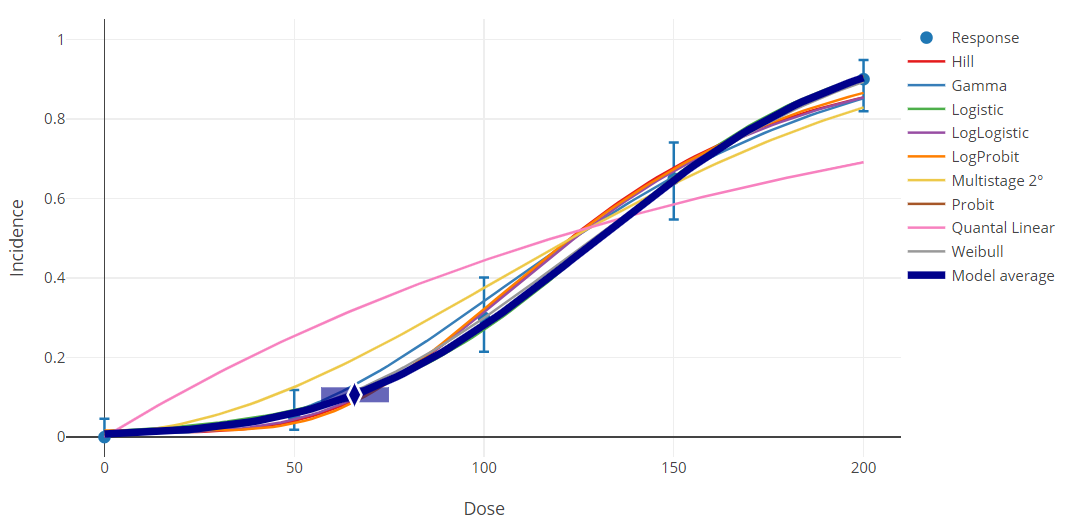
Figure 105. Sample Bayesian dichotomous results plot.

Bayesian Dichotomous Model Descriptions

Note

At this time, EPA does not offer technical guidance on Bayesian modeling or Bayesian model averaging.

From a Bayesian perspective, inference proceeds by defining a data-generating mechanism, given a model, \(M\), and its parameters. For our purposes, \(M\) would be one of the models listed in Dichotomous Response Models that determines the probability of response. For the dichotomous models, the data-generating mechanism would be the assumption that the observations were obtained from binomial sampling, having the dose-dependent probability of response defined by one of those models (with specific values of the parameters in that model).

We can then relate that to the likelihood, here denoted \(\mathcal{l}(D|M)\), which shows explicitly that it is the likelihood of the data, \(D\), conditional on the model. The functional form of the log of the likelihood is presented in Likelihood Function.

The set of Bayesian dichotomous models used in BMDS Online is identical to the set of models used for maximum-likelihood estimation (MLE) approaches (Dichotomous Response Models). In the following, let \(\theta\) be the vector of parameters that are required to define the any one of those models. So, for example, for the Weibull model \(\theta = (g, \alpha, \beta)\). The additional consideration incorporated into the Bayesian approach is the specification of a prior distribution for \(\theta\). The Bayesian approach takes the specified prior and updates it using the data under consideration to obtain a posterior distribution for \(\theta\).

From a Bayesian perspective, functions of \(\theta\) also have posterior densities. So, using the equations (which express the BMD as function of the model parameters) summarized in Calculation of the BMD for Individual Dichotomous Models, one can derive a posterior distribution for the BMD.

BMDS summarizes the posterior for the BMD as follows. The BMD is equated to the value obtained by using the maximum a posteriori (MAP) \(\theta\) estimate. The MAP is the value of \(\theta\) that maximizes the posterior log-likelihood. The posterior density is itself approximated using a Laplacian approximation. This approximation is also used to estimate BMDL and BMDU values, which are the percentiles from that density that correspond to the confidence level selected by the user.

The priors for the BMDS dichotomous models are defined below.

Note

The priors for the parameters are based on scaled doses and scaled responses; BMDS performs this scaling automatically.

BMDS automatically scales the doses by dividing by the maximum dose in the dataset under consideration, i.e., that the doses under consideration range from 0 to 1 (inclusive). BMDS automatically scales the responses by dividing by the mean response in the control (or lowest dose) group.

The user does not need to scale anything beforehand. That means that the parameter estimates, and BMD values returned by the program have been adjusted back to the original scale of the doses and the original scale of the responses specified in the input data file.

Bayesian Dichotomous Models and their Respective Parameter Priors

Multistage

Model Form

\[p(dose) = g + (1 - g)\left( 1 - \exp\left\lbrack - \sum_{i = 1}^{n}{\beta_{i}dose^{i}} \right\rbrack \right)\]

Parameters

\(g\) = background

\(\beta_{i}\) = dose coefficients

Parameter Constraints

\(0\ \leq \ g\ < \ 1\)

\(\beta_{i} > 0\)

\(N \geq 2\)

Priors

\(logit(g) \sim Normal(0,2)\)

\(\alpha \sim Normal(0,1)\)

\(\beta \sim Lognormal(\ln(2),0.5)\)

Notes

The prior over \(\beta_{1}\) reflects the belief that the linear term should be strictly prositive if the quadratic term is positive in the two-hit model of carcinogenesis. The difference in priors between the Multistage and Quantal Linear models is by design. The objective is to emphasize the higher-order terms in each model. The Multistage 1 model uses a prior favoring shallow dose-response relationships, while the Quantal Linear model uses a more diffuse prior.

For model averaging purposes, \(N = 2\).

Weibull

Model Form

\[p(dose) = g + (1 - g)\left( 1 - \exp\left\lbrack - \beta{dose}^{\alpha} \right\rbrack \right)\]

Parameters

\(g\) = background

\(\alpha\) = power

\(\beta\) = slope

Parameter Constraints

\(0\ \leq \ g\ < \ 1\)

\(-40\ < \ \alpha\ \leq \ 40\)

\(0\ < \ \beta < \ 10,000\)

Priors

\(logit(g) \sim Normal(0,2)\)

\(\alpha \sim Lognormal(\sqrt(0.18),0,5)\)

\(\beta \sim Lognormal(0,1.5)\)

Quantal Linear

Model Form

\[p(dose) = g + (1 - g)\left( 1 - \exp\left\lbrack - \beta{dose} \right\rbrack \right)\]

Parameters

\(g\) = background

\(\beta\) = slope

Parameter Constraints

\(0\ \leq \ g\ < \ 1\)

\(0\ < \ \beta < \ 10,000\)

Priors

\(logit(g) \sim Normal(0,2)\)

\(\beta \sim Lognormal(0,1)\)

Notes

The difference in priors between the Quantal Linear model and the Multistage 1 model is by design. The objective is to emphasize the higher-order terms in each model. The Quantal Linear model is not the same as the Multistage 1 model. This is important for model averaging purposes. The Multistage 1 model uses a prior favoring shallow dose-response relationships, while the Quantal Linear model uses a more diffuse prior.

Gamma

Model Form

\[p(dose) = g + \frac{1 - g}{\Gamma(\alpha)}\int_{0}^{\beta d}{t^{\alpha - 1}\exp( - t)dt\ }\]

Parameters

\(g\) = background

\(\alpha\) = power

\(\beta\) = slope

Parameter Constraints

\(0\ \leq \ g\ < \ 1\)

\(0.2\ < \ \alpha\ \leq \ 20\)

\(0\ < \ \beta\ < 10,000\)

Priors

\(logit(g) \sim Normal(0,2)\)

\(\alpha \sim Lognormal(\ln(2)\sqrt(0.18))\)

\(\beta \sim Lognormal(0,1)\)

Notes

The prior for \(\alpha\) entails that there is only a 0.05 prior probability the power parameter will be less than 1. This allows for models that are supralinear; however, it requires a large amount of data for the \(\alpha\) parameter to go much below 1.

The \(\alpha\) parameter is also constrained to be greater than 0.2 for numerical reasons.

Logistic

Model Form

\[p(dose) = \frac{1}{1 + exp\lbrack - \alpha - \beta(dose)\rbrack}\]

Parameters

\(\alpha\) = intercept

\(\beta\) = slope

Parameter Constraints

\(- 20 < \alpha < 20\)

\(0 < \ \beta\ < 40\)

Priors

\(\alpha \sim Normal(0,2)\)

\(\beta \sim Lognormal(0,2)\)

Log-Logistic

Model Form

\[p(dose) = g + \frac{1 - g}{1 + exp\lbrack - \alpha - \beta log(dose)\rbrack}\]

Parameters

\(g\) = background

\(\alpha\) = power

\(\beta\) = slope

Parameter Constraints

\(0\ \leq \ g\ < \ 1\)

\(- 40\ < \ \alpha\ \leq \ 40\)

\(0\ < \ \beta < 20\)

Priors

\(logit(g) \sim Normal(0,2)\)

\(\alpha \sim Normal(0,1)\)

\(\beta \sim Lognormal(\ln(2),0.5)\)

Probit

Model Form

\[p(dose) = \ \Phi(\alpha + \ \beta dose)\]

where

\(\Phi(x) = \int_{- \infty}^{x}{\phi(t)dt}\)

and

\(\phi(t) = \ \frac{1}{\sqrt{2\pi}}e^{\frac{- t^{2}}{2}}\)

Parameters

\(\alpha\) = intercept

\(\beta\) = slope

Parameter Constraints

\(- 20 < \alpha < 20\)

\(0\ < \ \beta < 40\)

Priors

\(\alpha \sim Normal(0,2)\)

\(\beta \sim Lognormal(0,1)\)

Notes

\(\Phi\) is the standard Normal cumulative distribution function, \(\phi\) is the standard Normal density function.

Log-Probit

Model Form

\[p(dose) = g + (1 - g)\Phi\left\lbrack \alpha + \beta\log(dose) \right\rbrack\]

where

\(\Phi(x) = \int_{- \infty}^{x}{\phi(t)dt}\)

and

\(\phi(t) = \ \frac{1}{\sqrt{2\pi}}e^{\frac{- t^{2}}{2}}\)

Parameters

\(g\) = background

\(\alpha\) = intercept

\(\beta\) = slope

Parameter Constraints

\(0\ \leq \ g\ < \ 1\)

\(- 40\ \leq \alpha < 40\)

\(0\ < \ \beta\ \leq 20\)

Priors

\(logit(g) \sim Normal(0,2)\)

\(\alpha \sim Normal(0,1)\)

\(\beta \sim Lognormal(\ln(2),0.5)\)

Notes

\(\Phi\) is the standard Normal cumulative distribution function, \(\phi\) is the standard Normal density function.

Dichotomous Hill

Model Form

\[p(dose) = g + \frac{(v - vg)}{1 + exp( - \alpha - \beta\log(dose))}\]

Parameters

\(g\) = background

\(v\) = maximum extra risk

\(\alpha\) = intercept

\(\beta\) = slope

Parameter Constraints

\(0\ \leq \ g\ < \ 1\)

\(- 40\ < \ v\ \leq 40\)

\(- 40\ < \alpha\ \leq 40\)

\(0\ < \ \beta\ \leq 40\)

Priors

\(logit(g) \sim Normal(-1,2)\)

\(\alpha \sim Normal(-3,3.33)\)

\(\beta \sim Lognormal(\ln(2),0.5)\)

\(logit(v) \sim Normal(0,3)\)

Note

For all the models described above, \(\text{logit}(g) = \ln\left( \frac{g}{1 - g} \right)\). \(Normal(x, y)\) denotes a Normal distribution with mean \(x\) and standard deviation \(y\). \(Lognormal(w, z)\) denotes a Lognormal distribution with log-scale mean \(w\) and log-scale standard deviation \(z\). Further, the background parameter constraints above are on the logit scale, which is the form in which BMDS uses these constraints for calculation. The constraints are input into the software on the real number scale, with values of -18/18 for the MLE model and -20/20 for the Bayesian model minimum/maximum. The software then performs a logit transformation on these values. The background parameter values output by BMDS in the results will have a range of 0 to the maximum dose for each model.

As the number of observations in a dataset increases, there should be less quantitative difference between the parameters and BMDs obtained from the Bayesian approach and from the maximum-likelihood estimation (MLE) approach.

When there are fewer data points, the priors will affect the Bayesian estimation. The impact may be most noticeable when the data suggest a “hockey-stick” shaped dose-response relationship, or when those data suggest strong supralinear behavior. In these cases, the priors specified above for the Bayesian approach will tend to “shrink back” parameter estimates to obtain smoother dose-response relationships where changes in the slope are more gradual.