Continuous Endpoints
Continuous endpoints take on values that are real numbers (as opposed to integers, for example), measuring things that can vary continuously (weights, concentrations, etc.).
The three key features of such measures that need to be specified to estimate a BMD are:
What direction of change indicates a toxic response (see Adverse Direction),
Definition of the BMD relative to the change in the response (see Benchmark Response), and
How the responses are distributed (see Distribution and Variance).
With respect to the distribution, one needs to consider the type of distribution and the nature of the variability around the center of the distribution. The options available to the user, discussed in Distribution and Variance, relate to all those choices.
This section provides details on the following topics:
Implementation of continuous models in BMDS
Entering continuous model data
Continuous model options
Options for restricting values of certain model parameters
Continuous Response Models
All the traditional maximum-likelihood estimation (MLE) models and options that were available for analyzing continuous response data in previous versions of BMDS are available in BMDS Online.
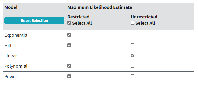
Figure 63. Default selection of continuous models on BMDS Online’s Settings tab.
Also available for all continuous models are options for Hybrid-Extra Risk and Hybrid-Added Risk benchmark responses (BMRs; see Options related to continuous BMR type and BMRF), and the Lognormal response distribution assumption (only available for Exponential models).
The user can choose to run the Hill, Polynomial, and Power models either restricted or unrestricted; the Linear model is not restricted while the Exponential models can only be run restricted.
Entering Continuous Response Data (Data Tab)
A BMDS analysis can have the following number of continuous datasets:
BMDS Online: A maximum of six datasets.
BMDS Desktop: No limit essentially; but it is recommended to create multiple analyses instead of putting large numbers of datasets into a single analysis.
pybmds: No limit.
For details on inserting or importing datasets, refer to Specifying Datasets.
For summarized continuous response data, the default column headers are Dose, N, Mean and Std. Dev.
For individual continuous response data, the default column headers are Dose and Response.
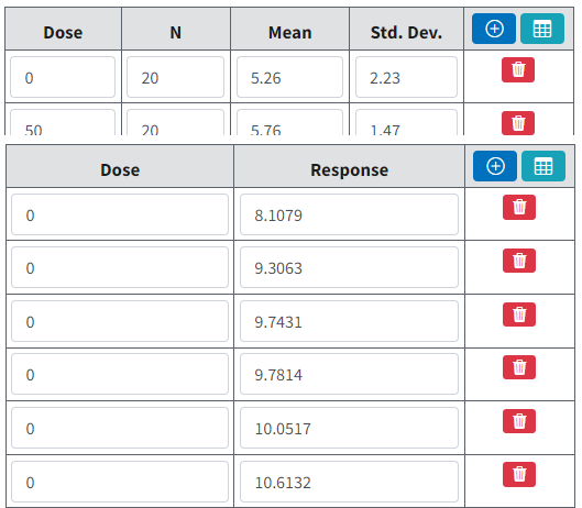
Figure 64. Default column headers for summarized data (top) and individual data (bottom)
Dataset Specifications (Settings Tab)
Datasets for an analysis can be a mix of individual and summarized data. Select a dataset’s Enabled checkbox to include it in the analysis.
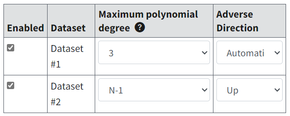
Figure 65. Dataset specification settings, with Enabled checkboxes selected.
Maximum Polynomial Degree
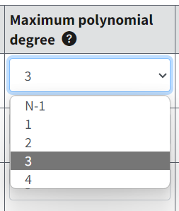
Figure 66. Maximum polynomial degree selections.
The default value for the maximum polynomial degree is the lesser of N-1 or 3, but the user can change this value to a higher number of degrees up to the lesser of N-1 or 8.
Hover the pointer over the question mark to display the following help text:
Note
Studies have indicated that higher degree polynomial models are not warranted in that they generally do not sufficiently improve fit over simpler models (Nitcheva et al., 2007; PMC2040324). Complex models also increase computing processing time and the chance of model failure.
Adverse Direction
Choices for the Adverse Direction option are Automatic (default), Up, or Down.
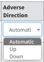
Figure 67. Adverse Direction picklist for the selected dataset.
This option refers to whether adversity increases as the dose-response curve rises “up” or falls “down.” Manually choose the adverse direction if the direction of adversity is known for the endpoint being studied.
If Automatic is chosen, BMDS chooses the adverse direction based on the shape of the observed dose-response relationship.
This selection only affects how the user-designated benchmark response (BMR) is used in conjunction with model results to obtain the BMD.
Option Sets
On the BMDS Online Settings tab, the user can define up to six Option Sets to apply to multiple user-selected models and multiple user-selected datasets in a single batch process. (There is no limit on option sets in BMDS Desktop and pybmds.)
Select the blue Plus button to add a new Option Set row. Select the red Trashcan button to delete that Option Set row.
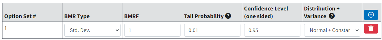
Figure 68. Continuous Model Option Set row.
Defining the BMD
The following options are related to the definition of the BMD and its bounds:
Benchmark Response (BMR) Type, which defines the method of choice for determining the response level used to derive the BMD (i.e., relative deviation, standard deviation, etc.). For details on these methods, refer to the Options related to continuous BMR type and BMRF dropdown.
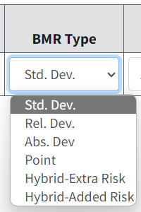
Figure 69. BMR Type picklist selections.
The BMRF (Benchmark Response factor) is specific to the method selected for the BMR Type. The Options related to continuous BMR type and BMRF dropdown summarizes the options related to BMR Type and BMRF.
Tail Probability marks the cut-off for defining adversity and applies only to Hybrid-Extra Risk BMR Type, not the background rate. If the default setting of 0.01, for example, is used, this indicates that the user has specified that, in the absence of exposure, there is a probability of 1% for a response that is considered adverse. This is a “tail probability” in the sense that it specifies how much of the tail of the distribution of responses (upper or lower) is in the adverse range. It implicitly defines the cut-off between Normal and adverse responses. The user can edit the value for this setting.
Confidence Level is set to 0.95 by default. This confidence level corresponds to a one-sided confidence bound, in either direction. In other words, if the confidence level is set to 0.95, the BMDL is the one-sided 95% lower bound on the BMD; the BMDU is the one-sided 95% upper bound on the BMD. The interval from the BMDL to the BMDU would, in that case, be a 90% confidence interval.
Distribution and Variance
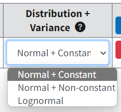
Figure 70. Distribution and Variance picklist selections.
The underlying data distribution and the variability around the center of that distribution are linked options.
In total, three combinations are allowed:
Normal distribution, constant variance (default): each dose group has the same variance, which is estimated by BMDS along with the dose-response model parameters.
Normal distribution, non-constant (modeled) variance: each dose group may have a different variance, described by a variance model (see Likelihoods of Interest Table) with two parameters (α and ρ) relating the dose group’s estimated mean value (see below) to the variance. Those two parameters are estimated simultaneously with the parameters of the dose-response model.
Important
The \(\alpha\) parameter is returned for all models except for the exponential models, which return \(ln(\alpha).\)
Lognormal distribution, constant coefficient of variation (CV): for lognormally distributed responses, each dose group has the same CV, which entails that the log-scale variance is constant over dose groups (though the natural-scale variance will differ from group to group).
Important
CV = standard deviation divided by mean. Log-scale refers to the values of the logarithms of the responses. Natural-scale refers to the values of the responses, untransformed.
With respect to the response distribution (Normal or Lognormal), please note the following:
The Lognormal distribution can only be assumed when the responses are strictly positive. The Lognormal distribution is only applicable to positive real values.
Regardless of the distribution assumed, the dose-response model under consideration is the representation of the change in the median of the distribution of responses as a function of dose. If we denote the median at dose d by \(m(d)\), then it is always true for BMDS that \(m(d) = f(d)\), where \(f(d)\) is the dose-response function under consideration (see Continuous Dose-Response Models and Parameters).
If the assumed data distribution is Normal, then it is also true that the mean at dose d, \(μ(d)\), is equal to the median. Thus, it is common under the Normal assumption to describe the dose-response function as a model of the mean response, and to write \(μ(d) = f(d)\), where \(f(d)\) is again one of the dose-response functions described in Continuous Dose-Response Models and Parameters.
When modeling continuous response data, the standard assumption for the BMDS continuous models is that the underlying distributions (one for each dose group) are Normal, with a mean given by the dose-response model and a variance as specified by the user (constant or a function of the mean response). An alternative assumption is that the responses are lognormally distributed.
In BMDS, all continuous models allow the user to choose between Normal response distribution assumptions; whereas the Lognormal response distribution is only available for Exponential models.
If the user has access to the individual response data, those data can be log-transformed prior to analysis but, as discussed below, this is not a recommended approach. If the user suspects that the responses are lognormally distributed, the recommended approach is to model the untransformed data assuming the underlying distribution is Lognormal with median values defined by the dose-response function and a constant log-scale variance, corresponding to an assumption of a constant CV.
Exact and Approximate MLE Solutions
The exact MLE solution cannot be obtained when the data are assumed to be Lognormally distributed and the data are presented in terms of group-specific means and standard deviations. In that case, the results are approximate MLE solutions. The means (\(m_{L}\)) and standard deviations (\(s_{L}\)) of the log-transformed data are estimated as follows:
estimated log-scale sample mean (\(m_{L}\)): \(m_{L} = \ln{(m) - \frac{s_{L}^{2}}{2}}\)
estimated log-scale sample standard deviation (\(s_{L}\)): \(s_{L} = \sqrt{(\ln\left\lbrack 1 + \frac{s^{2}}{m^{2}} \right\rbrack)}\)
where m and s are the sample mean and sample standard deviation, respectively.
When data are assumed to be lognormally distributed and individual response data are available, BMDS provides an exact maximum-likelihood estimation (MLE) solution. In BMDS, the exact solution is the only solution option implemented when individual observations are input, and the Lognormal assumption is chosen. BMDS does not provide an option for computing the approximate solution.
If the user wants to compute an approximate solution from individual observations (e.g., for research purposes), then they should use the following procedure:
Compute the group-specific sample means and sample standard deviations.
Input those values as would be done for an analysis based on those summary statistics (but still selecting Lognormal as the distribution type).
Log-transformed Responses are NOT Recommended
Warning
Using log-transformed responses in the analysis is not recommended.
If the user chooses to log-transform the data prior to analysis, then the interpretation of the BMD and BMDL estimates would have to be considered carefully (and perhaps in consultation with a statistician). Data interpretation when using log-transformed responses will not be the same as when using the natural-scale response values. Indeed, the models—when “transformed back” to the natural scale—will not correspond to any of the standard BMDS models.
For example, if using the power model on log-transformed responses, the user is actually implicitly modeling the medians (on the natural-scale) with the function \(e^{(background + slope \times {dose)}^{power}}\) which is not a standard BMDS model and whose characteristics (e.g., exponential increases in response) may not be those desired by the user.
Similarly, the interpretation of the BMD will not correspond to simple expressions (e.g., if the BMR is set equal to a relative deviation of 10%, that relative deviation will be assessed on the log-scale and so will not yield BMD or BMDL estimates that correspond to a 10% change in the original mean responses).
For these reasons, log-transforming the response values is not considered a best practice and, as stated, should only be applied and interpreted with supporting statistical expertise.
Therefore, in most cases, the user should use non-transformed values and select the Lognormal distribution if the data are assumed to be lognormally distributed.
Specific Continuous Results
Goodness of Fit Table
The Goodness of Fit table displays the model predictions relative to the observed (or calculated) data that were used as input, one row for each dose group. Generally, one desires to have the model predictions match the input data as well as possible.
Note that in the Goodness of Fit tables shown in Figure 71. and Figure 72.:
Sample Mean = the sample mean for both Normally and Lognormally distributed data.
Approximate Sample Median = the median computed from the observed data. In the case of Lognormally distributed responses, the median is calculated as \(exp(z_{L})\), where \(z_{L}\) is the log-scale mean, estimated if need be for summarized response data as shown in Distribution and Variance.
Model Fitted Mean/Median = model-predicted median, which equals the mean in the case of Normally distributed data.
Sample SD = the standard deviation computed from the observed data. In the case of Normally distributed data, this equals the sample standard deviation of the responses.
Approximate Sample GSD = the standard deviation (or geometric standard deviation, in the case of Lognormally distributed data) computed from the observed data. In the case of Lognormally distributed data, this equals \(exp(s_{L})\), where \(s_{L}\) is the log-scale standard deviation, estimated if need be for summarized response data as shown in Distribution and Variance.
Model Fitted [G]SD = the standard deviation (or geometric standard deviation, in the case of Lognormally distributed data) estimated by the model.
Scaled Residual = For Normal responses, the scaled residual equals:
\[(Sample\ Mean\ - \ Model\ Fitted\ Mean)/(Model\ Fitted\ SD/\sqrt{N_{i}})\]Whereas, for Lognormal responses, the scaled residual equals:
\[(ln(Sample\ Median)\ - \ ln(Model\ Fitted\ Median))/(ln(Model\ Fitted\ GSD)/\sqrt{N_{i}})\]
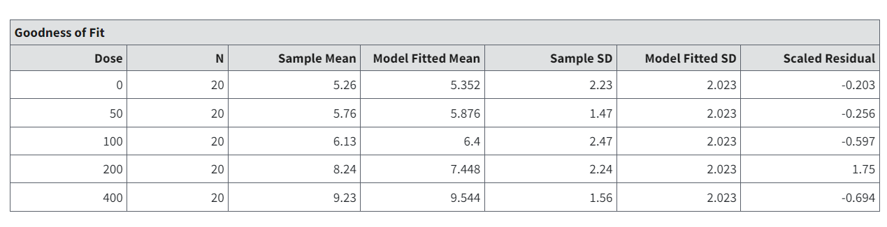
Figure 71. Goodness of Fit table headings, with Normal assumption.
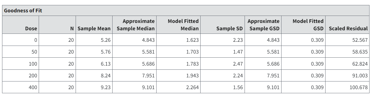
Figure 72. Goodness of Fit table headings, with Lognormal assumption. Note the column header similarities/differences between the two tables.
The scaled residual value is a calibrated difference between the observations and the model predictions. Regardless of the assumption about the distribution of the responses, it is computed on the scale corresponding to the Normal distribution. Moreover, the denominator for its calculation estimates the degree of uncertainty (standard error of the mean) for the model prediction. Therefore, scaled residual values greater than about 2 in absolute value are indicative of mismatches between predicted and observed values that may indicate poorer fit, at least locally.
Likelihoods of Interest Table
The Likelihoods of Interest table displays the log-likelihoods, number of parameters, and AIC for five models, including the dose-response model under consideration (i.e., fitted).
BMDS uses likelihood theory to estimate model parameters and ultimately to make inferences based on dose-response data. Maximum likelihood is the process of estimating the model parameters; the likelihood function is as large as possible (maximized) given the form of the model under consideration and the data. In other words, parameter values are “chosen” such that the subject model (e.g., polynomial or power) obtains the best possible fit to the data, given the constraints of the model’s parameter structure.
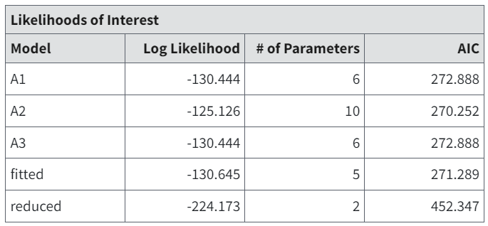
Figure 73. Likelihoods of Interest table.
The number of parameters for each model excludes parameters that have values on one of the bounds set for their estimation (either bounds specified by the user or those inherent constraints associated with the model; see Continuous Dose-Response Models and Parameters).
Important
The likelihood is maximized given bounds on parameters. As a result, it is technically not guaranteed to be the universal MLE, but rather a bounded MLE.
The five log-likelihood models can be used for tests of hypotheses, including tests of fit, that are asymptotically Chi-square. Each of these log-likelihood values corresponds to a model the user may consider in the analysis of the data.
Likelihood Values and Models for Continuous Endpoints
Model A1 estimates separate and independent means for the observed dose group (it is full or saturated in that respect) but posits a constant variance over those groups
Description:
\(Y_{ij} = \mu_{i} + e_{ij}\)
\({Var\{ e}_{ij}\} = \sigma^{2}\)
Model A2 is the fullest model in that it estimates separate and independent means for the observed dose groups (as in Model A1) and it also estimates separate and independent variances for those groups. There is no assumed functional relationship among the means or among the variances across dose groups. This model is often referred to as the “saturated” model (it has as many mean and variance parameters as there are dose groups). The log-likelihood obtained for this model is the maximum attainable, for the data under consideration.
Description:
\(Y_{ij} = \mu_{i} + e_{ij}\)
\({Var\{e}_{ij}\} = {\sigma_{i}}^{2}\)
Model A3 is similar to model A2 and may only differ with respect to its variance parameters. Model A2 estimates separate and independent means for the observed dose groups (like A1). If the user specifies a constant variance for the fitted model, then model A3 will also assume that, and it becomes identical to Model A1. If the user assumes a non-constant variance for the fitted model, then Model A3 will also assume the same functional form for the variance.
Description:
\(Y_{ij} = \mu_{i} + e_{ij}\)
\({Var\{ e}_{ij}\} = \alpha \times {\mu_{i}}^{\rho}\)
The fitted model is the user-specified model (e.g., power or polynomial, among others). A user may have reason to believe that a certain model may describe the data well, and thus uses it to calculate the BMD and BMDL.
Description:
The user-specified model
The reduced model (R) is the model that implies no difference in mean or variance over the dose levels. In other words, it posits a constant mean response level with the same variance around that mean at every dose level.
Description:
\(Y_{i} = \mu + e_{i}\)
\({Var\{ e}_{i}\} = \sigma^{2}\)
Tests of Mean and Variance Fits
The Tests of Mean and Variance Fits table show the results of four tests based on the log-likelihoods from the Likelihoods of Interest table. The p-values associated with the tests are based on asymptotic properties of the likelihood ratio.
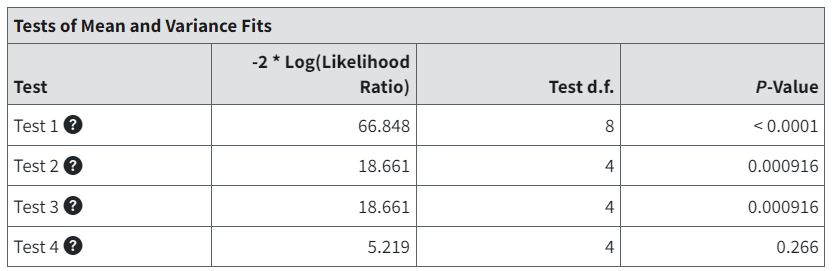
Figure 74. Test of Means and Variance Fits table.
The likelihood ratio is the ratio of two likelihood values, many of which are given in the BMDS output. Statistical theory proves that \(- 2*ln(likelihood\ ratio)\) converges to a Chi-square random variable as the sample size gets large and the number of dose levels gets large. These values can in turn be used to obtain approximate probabilities to make inferences about model fit. Chi-square tables can be found in almost any statistical reference book.
Suppose the user wishes to test two models, A and B, for fit. One assumption that is made for these tests is that model A is nested within Model B, i.e., that Model B can be simplified (via restriction of some parameters in Model B) in such a way that the simplified model is Model A. This implies that Model A has fewer varying parameters. As an example, consider that the linear model is a “simpler” or “nested” model relative to the power model because the linear model has the power parameter restricted to be equal to 1.
Note
The model with a higher number of parameters is always in the denominator of this ratio.
Suppose that \(L(X)\) represents the likelihood of model X. Now, using the theory, \(- 2 \times ln\{\frac{L(A)}{L(B)}\}\) approaches a Chi-square random variable. This can be simplified by using the fact that the log of a ratio is equal to the difference of the logs:
The values in the Likelihoods of Interest table are in fact the log-likelihoods, as discussed above, \(\ln\{ L(B)\}\) and \(\ln\{ L(A)\}\), so this likelihood ratio calculation becomes just a subtraction problem. This value can then in turn be compared to a Chi-square random variable with a specified number of degrees of freedom.
As mentioned in conjunction with the Likelihoods of Interest table, each log-likelihood value has an associated number of parameters. The number of degrees of freedom for the Chi-square test statistic is merely the difference between the two model parameter counts of the two models. In the mini-example above, suppose Model A has 5 fitted parameters, and that Model B has 8. In this case, the Chi-square value to be compared to would be a Chi-square with 8 - 5 = 3 degrees of freedom.
In the A vs B example, what is exactly being tested? In terms of hypotheses, it would be:
H0: A models the data as well as B
H1: B models the data better than A
Keeping these tests in mind, suppose \(2 \times \log\{ L(B)\}\ - \ 2 \times \log\{ L(A)\}\ = \ 4.89\) based on 3 degrees of freedom. Also, suppose the rejection criteria is a Chi-square probability of less than 0.05. Looking on a Chi-square table, 4.89 has a p-value somewhere between 0.10 and 0.25. In this case, H0 would not be rejected, and it would seem to be appropriate to model the data using Model A (i.e., the simpler model A models the data as well as the more complex model B). BMDS automatically does the table look-up for the user and provides the p-value associated with the calculated log-likelihood ratio having degrees of freedom as described above.
The Tests of Means and Variance table in BMDS provides four default tests for any of the continuous models.
Test 1 (A2 vs R): Tests the null hypothesis that responses and variances do not differ among dose levels. If this test fails to reject the null hypothesis, there may not be a dose-response.
This test compares Model R (the simpler model) to Model A2. Model R is a simpler A2 (or nested within A2) since R can be obtained from A2 by restricting all the mean parameters to be equal to one another and restricting all the variance parameters to be equal to one another. If this test fails to reject the null hypothesis, then there may not be a dose-response, as the inference would be that the simpler model (R) is not much worse than the saturated model. The default p-value for the test (as reported in the Tests of Interest section of the output) is 0.05. A p-value less than 0.05 is an indication that there is a difference between response and/or variances among the dose levels and supports a conclusion to model the data. A p-value greater than 0.05 is an indication that the data may not be suitable for dose-response modeling.
Test 2 (A1 vs A2): Tests the null hypothesis that variances are homogeneous. If this test fails to reject the null hypothesis, the simpler constant variance model may be appropriate.
This test compares A1 (the simpler model) to Model A2. Model A1 is a simpler A2 (or nested within A2) since A1 can be obtained from A2 by restricting all the variance parameters to be equal to one another. If this test rejects the null hypothesis, the inference is that the constant variance assumption is incorrect and a modeled variance is necessary to adequately represent the data. The default p-value for rejecting the null hypothesis is 0.05 (as reported in the Tests of Interest section of the output). A p-value less than 0.05 is an indication that the user should consider running a non-homogeneous (e.g., nonconstant) variance model. A p-value greater than 0.05 is an indication that a constant variance assumption may be suitable for the dose-response modeling.
Test 3 (A3 vs A2): Tests the null hypothesis that the variances are adequately modeled. If this test fails to reject the null hypothesis, it may be inferred that the variances have been modeled appropriately.
Here, the test is one to see if the user-specified variance model, is appropriate. If the user-specified variance model is Constant Variance, then Models A1 and A3 are identical; this test is the same as Test 2, with the same interpretation. If the user-specified variance model is nonconstant (\({\sigma_{i}}^{2} = \alpha \times {\mu_{i}}^{\rho}\)), this test determines if that equation appears adequate to describe the variance across dose groups. Model A3 is the simpler version of Model A2 obtained by constraining the variances to fit the nonconstant variance equation. The default p-value for rejecting the null hypothesis is 0.05 (as reported in the Tests of Interest section of the output). A p-value less than 0.05 is an indication that the user may want to consider a different variance model. A p-value greater than 0.05 supports the use of user-specified variance model for the dose-response modeling.
Test 4 (Fitted vs A3): Tests the null hypothesis that the model for the mean fits the data. If this test fails to reject the null hypothesis, the user has support for the selected model.
This test compares the Fitted Model to Model A3. The Fitted Model is a simpler Model A3 (or nested within Model A3) because it can be obtained by restricting the means (unrestricted in A3) to be described by the dose-response function under consideration. If this test fails to reject the null hypothesis, the inference is that the fitted model is adequate to describe the dose-related changes in the means (conditional on the form of the variance model; the form of the variance model is the same for the Fitted Model and Model A3). Failure to reject the null hypothesis is associated with the inference that the restriction of the means to the shape of the dose-response function under consideration is adequate. The default p-value for rejecting the null hypothesis is 0.1 (as reported in the Tests of Interest section of the output). A p-value less than 0.1 is an indication that the user may want to try a different model (i.e., the fit of the Fitted Model is not good enough). A p-value greater than 0.1 is an indication that the Fitted Model appears to be suitable for dose-response modeling.
Plot and Error Bar Calculation
The graphical output, i.e., plot, is a visual depiction of the results of the modeling. Although plot features are common to all models, here we describe the one additional detail specific to the continuous models, i.e., computation of the error bars for mean response of the dose group:
The plotting routine calculates the standard error of the mean (SEM) for each group. The routine divides the group-specific observed variance (obs standard deviation squared) by the group-specific sample size.
The routine then multiplies the SEM by the Student-T percentiles (2.5th percentile or 97.5th percentile for the lower and upper bound, respectively) appropriate for the group-specific sample size (i.e., having degrees of freedom one less than that sample size). The routine adds the products to the observed means to define the lower and upper ends of the error bar.
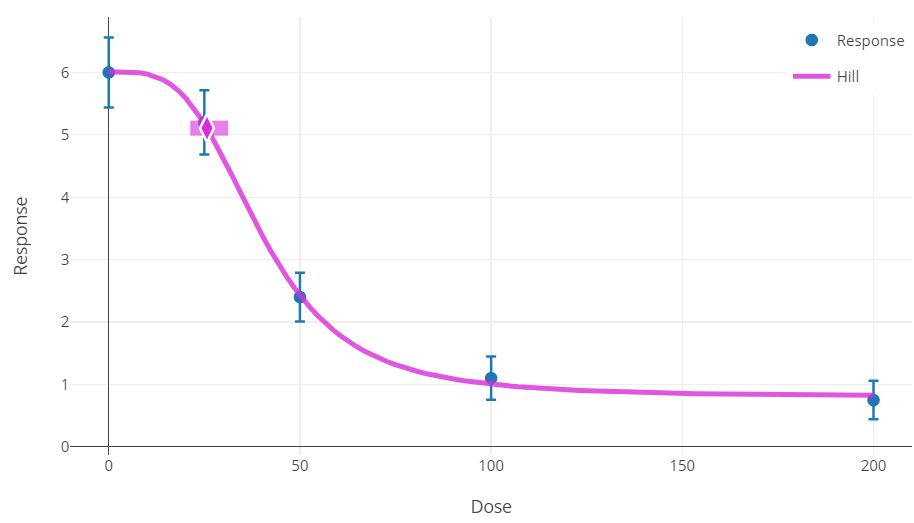
Figure 75. Maximum likelihood approach results plot for continuous data.
Mathematical Details for Models for Continuous Endpoints in Simple Designs
Models in this section are for continuous endpoints, such as weight or enzyme activity measures, in simple experimental designs that do not involve nesting or other complications. The models predict the median value of the response, \(m(dose)\), expected for a given dose and the variation around that median.
As evidenced by the previous discussion of the options available for continuous models, modeling of continuous endpoints requires consideration of more details than do those for dichotomous endpoints in similar designs. This section presents the mathematical and statistical details that determine how estimation is accomplished in BMDS.
Continuous Dose-Response Models and Parameters
The definitions of the continuous models are fully specified below. Note that \(m(dose)\) is the median response for the dose level specified.
Model Form
The Linear model is a form of the polynomial model.
\(n\ \)is the degree of the polynomial, specified by user and must be a positive integer (maximum value = 8)
Parameters
\(g\) = control response (intercept)
\(\beta_{0}\ldots\beta_{n}\): polynomial coefficients
Parameter Constraints
None.
User Parameter Restriction Options
Restrict the value of the polynomial coefficients to be either non-positive or non-negative guarantees that the resulting function will be strictly decreasing, strictly increasing, or perfectly flat (when all the coefficients are zero). If the coefficients are unrestricted (i.e., an unrestricted form of the model is run), then more complicated shapes are possible, and, particularly as the degree of the polynomial approaches the number of dose groups minus one, the polynomial will often be quite wavy.
Model Form
The Linear model is a form of the polynomial model.
Parameters
\(g\) = control response (intercept)
\(\beta\) = slope
Parameter Constraints
None.
User Parameter Restriction Options
None.
Model Form
Parameters
\(g\) = control response (intercept)
\(v\) = slope
\(n\)= power
Parameter Constraints
0 ≤ \(n\) ≤ 18
User Parameter Restriction Options
\(n\) may be further restricted to values ≥ 1.
Notes
If \(n\) < 1, then the slope of the dose-response curve becomes infinite at the control dose. This is biologically unrealistic and can lead to numerical problems when computing confidence limits, so several authors have recommended restricting \(n\) ≥ 1.
Note that the upper bounds for the power parameter in the Power model have been set to 18. That value was selected because it represents a very high degree of curvature that should accommodate almost every dataset, even ones with very (or absolutely) flat dose-response at low doses followed by a very steep dose-response at higher doses.
Model Form
Parameters
\(g\) = control response (intercept)
\(k\) = dose with half-maximal change (normalized)
\(n\)= power
\(v\)= maximum change
Parameter Constraints
0 ≤ \(k\) ≤ 5
0 ≤ \(n\) ≤ 18
User Parameter Restriction Options
\(n\) may be further restricted to values ≥ 1.
Notes BMDL estimates from models that have an asymptote parameter (including the Hill model) can be unstable when a wide range of parameter values can give nearly identical likelihoods. One indicator of that problem is that the estimated asymptotic response is far outside the range of the observed responses. The user should consult a statistician if this behavior is seen or suspected.
Note that the upper bounds for the power parameter in the Hill model have been set to 18. That value was selected because it represents a very high degree of curvature that should accommodate almost every dataset, even ones with very (or absolutely) flat dose-response at low doses followed by a very steep dose-response at higher doses.
Model Form
Parameters
\(a\) = control response (intercept)
\(b\) = slope
\(c\)= asymptote term
\(d\)= power
Parameter Constraints
\(a\) > 0
0 < \(b\) < 100
\(c\) > 1 for responses increasing with dose
0 < \(c\) < 1 for responses decreasing with dose
1 ≤ \(d\) ≤ 18
Notes
The sign in “\(\pm b\)” (Exp2 and Exp3 models) will change depending on the user-designated or auto-detected direction of change:
+ for responses increasing with dose
- for responses decreasing with dose
BMDL estimates from models that have an asymptote parameter (including the Exponential5 model) can be unstable when a wide range of parameter values can give nearly identical likelihoods. One indicator of that problem is that the estimated asymptotic response is far outside the range of the observed responses. The user should consult a statistician if this behavior is seen or suspected.
Note that the upper bounds for the power parameter in the Exponential models have been set to 18. That value was selected because it represents a very high degree of curvature that should accommodate almost every dataset, even ones with very (or absolutely) flat dose-response at low doses followed by a very steep dose-response at higher doses.
Reference for Exponential models
RIVM (National Institute for Public Health and the Environment (Netherlands)). (RIVM, 2018). PROAST.
Variance Model
In addition to the model for the median response as a function of dose, the model for the variance also needs to be defined.
For responses assumed to vary Normally around the median, the variance model is:
where \(\alpha\) (> 0) and \(\rho\) are parameters estimated simultaneously with the parameters of the dose-response function (see Continuous Dose-Response Models and Parameters). As in the model equations, \(m\left( {dose}_{i} \right)\) is the predicted median (from the dose-response model under consideration) for the \(i^{th}\) dose group.
Note that when a constant variance model is specified by the user, the parameter \(\rho\) is set to 0 and only \(\alpha\) will be estimated. In that case,
When the responses are assumed to be Lognormally distributed, then the variance modeled is the log-scale variance:
Because, for Lognormal data, BMDS is restricted to a constant log-scale variance model (equivalent to a constant coefficient of variation), \(\rho\) does not appear in that equation (in essence, it is once again set to 0 under the assumption of Lognormally distributed responses).
The formulation of the variance model shown above allows for several commonly encountered situations. When the estimated value of \(\rho\ > 0\), the estimated variances will increase with increasing median values and decrease with decreasing median values. When \(\rho\ < 0\), the variances will decrease with increasing median values and increase with decreasing median values. If \(\rho\ = \ 1\), then the variance is proportional to the median. If \(\rho\ = \ 2\), then the coefficient of variation is constant, a common assumption especially for biochemical measures and one which mimics the constant coefficient of variation assumption of lognormally distributed responses (but without having to assume that the responses are in fact lognormally distributed).
Note
At this time, the change to the parameter restriction for the \(\rho\) parameter to allow negative values is only available in pybmds (version 25.2). Version 25.1 of pybmds, BMDS Online, and BMDS Desktop still restricts the \(\rho\) parameter to have values greater than or equal to zero, except for the Hill model.
Likelihood Function
Parameter estimates are derived by the method of maximizing the likelihood (i.e., they are maximum likelihood estimates, MLEs). The likelihood functions for the continuous responses are defined in this section.
Suppose there are G dose groups, having doses
with \(N_{i}\) subjects per dose group. Also suppose that \(y_{ij}\) is the measurement for the \(j^{th}\) subject in the \(i^{th}\) dose group. The form of the log-likelihood function depends upon whether the responses are assumed to be Normally or Lognormally distributed.
Assuming Normally Distributed Responses
For the assumption of Normally distributed responses, the log-likelihood function is:
where
\({\overline{y}}_{i} = \frac{\sum_{j = 1}^{N_{i}}y_{ij}}{N_{i}}\) (the sample mean for the \(i^{th}\) dose group),
\(s_{i}^{2} = \frac{\sum_{j = 1}^{N_{i}}{(y_{ij} - {\overline{y}}_{i})}^{2}\ }{N_{i} - 1}\) (the sample variance for the \(i^{th}\) dose group),
\(N = \ \sum_{i = 1}^{G}N_{i}\).
The parameters defining \(m\left( {dose}_{i} \right)\) and \({\sigma_{i}}^{2}\) (see previous two subsections) are optimized to maximize the LL equation value.
Assuming Lognormally Distributed Responses
For the assumption of Lognormally distributed responses, the log-likelihood function is:
where
\({\overline{z}}_{Li}\ = \ \)log-scale sample mean for \(i^{th}\) dose group, and
\({{\ s}_{Li}}^{2}\ = \ \)log-scale sample variance for \(i^{th}\) dose group.
As in the case of Normally distributed responses, the parameters defining \(m\left( {dose}_{i} \right)\) and \({\sigma_{Li}}^{2}\) (see previous two subsections) are optimized to maximize the LL equation value.
AIC and Model Comparisons
The Akaike Information Criterion (AIC) (Akaike, 1973) can be used to compare different models fit (by the same fitting method, e.g., by maximizing the likelihood) to the same dataset. The AIC is a statistic that depends on the value of LL (see previous section) and the number of estimated parameters, p:
\[AIC\ = \ - 2 \times LL\ + \ 2 \times p\]
Note that the AIC balances the goals of getting the highest LL value possible while being parsimonious with respect to the number of parameters needed to achieve a high LL value. Since the equation for AIC has a negative multiplier for LL (which one wants to be greater) and positive multiplier for p (which one wants to be as small as possible and still get good fit), a model with a smaller value of AIC than other models is presumed to be the better model based on AIC. Although such methods are not exact, they can provide useful guidance in model selection.
In BMDS, the number of estimated parameters includes only those that have not been estimated to equal a bounding value (either from the model-imposed constraints or user-imposed restrictions (see Continuous Dose-Response Models and Parameters).
Note
This counting process may or may not be reasonable, depending on the boundary value that a parameter in question hits.
For example, if the power parameter in a model hits (i.e., is estimated to be equal to) the upper bound of 18, it would usually be the case that one would want to count that parameter as one that is estimated, but BMDS Online does not do that.
For this reason, the user is apprised to carefully consider the cases where parameter bounds have been hit and to consider the implications for issues such as model comparison and model selection.
If a parameter hits a bound for any model, the parameter estimates are maximum likelihood estimates (MLEs) only in the restricted sense that the bounded parameter has been assigned a value and the other parameters are MLEs conditional on that assigned value. Such model results are not strictly comparable with others in terms of AIC. In such a case, the BMD and BMDL could depend on the choice of power parameter; thus, sensitivity analysis is recommended if one intends to rely on the reported BMD or BMDL. This is especially important when considering power parameters that have hit the upper bound of 18.
Note
To facilitate comparing models with different likelihoods (i.e., Normal vs. Lognormal), the log-likelihood is calculated using all the terms shown in the LL equations in Likelihood Function.
When comparing models having different parametric distributions, the AIC calculated using BMDS Online will result in the proper comparison between any two models regardless of underlying distribution.
Caution
A note of caution is required for situations where only the sample mean and sample standard deviation are available (summarized data) and for which the log-scale sample mean and sample standard deviation are only approximated when assuming lognormally distributed responses.
In such cases, the same approximations are made across all the dose-response models. It is therefore strictly valid to compare AIC results across any runs that assumed that the responses were Lognormally distributed.
However, comparisons of results where one set of results was obtained assuming Normality and one set was obtained assuming Lognormality should be made with caution.
In the latter case, if the AICs are similar (using that term loosely, because no specific guidance can be offered here), then the user ought not to base model selection on AIC differences. Selection when the AIC differences are larger may not be problematic, since the approximation used should not be too bad.
A conservative position would be that comparisons of model runs assuming Normally distributed responses to those assuming Lognormal responses should not be made using the AIC, if the underlying data are presented in summarized form (i.e., only sample means and sample standard deviations are available).
BMDL and BMDU Computation
The estimation of the BMDs, depending on the definition of the BMR type, is specified in the Options related to continuous BMR type and BMRF dropdown. The derivation of the confidence bounds for the BMD, i.e., the BMDL and BMDU, is defined in this section.
The general approach to computing the confidence limits for the BMD is the same for all the models in BMDS, and is based on the asymptotic distribution of the likelihood ratio (Crump and Howe, 1985).
Two different specific approaches are followed for the continuous models.
For the Power Model: For the power model, the equations that define the benchmark response in terms of the benchmark dose and the dose-response model are solved for one of the model parameters. The resulting expression is substituted back into the model equations, with the effect of re-parameterizing the model so that BMD appears explicitly as a parameter. A value for BMD is then found such that, when the remaining parameters are varied to maximize the likelihood conditional on that BMD value, the resulting log-likelihood is less than that at the maximum likelihood estimates by exactly
For the Polynomial, Hill, and Exponential Models: For the polynomial, Hill, and exponential models, it is impractical or impossible to explicitly reparameterize the dose-response model function to allow BMD to appear as an explicit parameter. For these models, the BMR equation is used as a non-linear constraint, and the minimum value of BMD is determined such that the log-likelihood is equal to the log-likelihood at the maximum likelihood estimates less
Occasionally, the following error message may appear for a model: BMDL computation is at best imprecise for these data. This is a flag that convergence for the BMDL was not successful in the sense that the required level of convergence (< 1e-3 relative change in the target function by the time the optimizer terminates) has not been achieved.
Continuous Response Data with Negative Means
Negative response data is defined as when the value of the mean or response is negative in the data.
Data with negative means should only be modeled with a constant variance model.
Avoid using the following models with negative response data:
Do not use exponential models with summarized negative response data. For exponential models, the mean cannot be negative.
Do not use power or exponential models with individual negative response data. For these models, the response cannot be negative.
Modeling Transformed Negative Data
It may occasionally be the case that, when modeling transformed data, the user will need to model negative data. In this case, the transformation used should be a variance-stabilizing transformation so that a constant-variance model would be appropriate.
If a standard deviation based BMR is used to define the BMD calculations, then a constant can be added to all the observations (or means) to make the values (means) positive. That will not change the standard deviations of the observations and would allow the user to model the variance.
Related topic: see Log-transformed Responses are NOT Recommended
Trend Test for Continuous Data
The Jonckheere-Terpstra trend test (Jonckheere, 1954; Terpstra, 1954) is a non-parametric statistical test used to detect a trend in continuous response data across ordered dose groups. The null hypothesis for the Jonckheere-Terpstra trend test is that the continuous response data are all from the same population, that is, the sample medians for all dose groups are equal. The alternative hypothesis is that the sample medians have an a priori ordering with at least one dose group sample being larger or smaller than the others. The test statistic counts, for each dose group, the number of times values in that group are greater than those in every lower order dose group and sums these counts across groups. A statistically significant tend can be inferred when the trend test p-value \(< 0.05\).
The Jonckheere-Terpstra trend test can be performed using a one-sided alternative hypothesis that the trend in responses is either increasing or decreasing (with the direction set by the user before running the test) or a two-sided alternative hypothesis used to detect a trend in either direction. Both exact and approximate versions of the Jonckheere-Terpstra trend test are available.
When running the Jonckheere-Terpstra trend test, the exact method, utilizing a permutation approach, is preferentially used. This permutation approach is not dependent on any distributional assumptions; it iteratively reshuffles the observed data (i.e., reshuffles the response data relative to dose group labels) to generate a dataset that might be expected due to chance. For each reshuffled (permuted) dataset, the test statistic is calculated and compared to the original test statistic. The final p-value is then the the proportion of permutted statistics that are greater than or lesser than the original statistic for decreasing and increasing trends, respectively. However, this exact method is only available when there are no ties in the data (i.e., there are no equal response values in the data set across dose groups) and when the total sample size is less than 150. The limit on sample size is based on the observation that computation time for the exact Jonckheere’s test increases in an exponential fashion with increasing total N:
Total Sample size (N) |
Computation Time (s) |
|---|---|
60 |
0.56 |
100 |
6.8 |
150 |
54 |
190 |
254 |
200 |
1026 |
When the total N exceeds 150 or ties in the data exist, the approximate approach, based on a normal approximation of the test statistics, is used instead. Users can opt to use the approximate approach even when there are no ties in the data and total N < 150.
Individual data are required for the Jonckheere-Terpstra trend test. If users only have summary level continuous data (i.e., means and standard deviations only), BMDS includes an approach to calculate synthetic individual response data that corresponds to the observed summary statistics. This is done by iteratively generating random samples using a normal distribution; random samples are generated until the sample mean and standard deviation match the target (i.e., observed) mean and standard deviation or until the maximum number of iterations are reached. If no sampled mean and standard deviation are found that match the target values, an error message is returned.
Note
At this time, the Jonckheere-Terpstra trend test is only available in pybmds (version 25.2). See pybmds Documentation for examples of usage