Nested Dichotomous Endpoints

In a nested study, for each dose tested, there is a group of experimental units receiving that specific dose of the chemical of interest. For each of those experimental units, several dichotomous observations are obtained, i.e., those dichotomous observations are nested within the experimental units.

Moreover, because of the nesting, one may suspect that the observations within each experimental unit are more similar to one another than they are to observations from other experimental units. For example, consider a developmental toxicity experiment, in which pregnant female rodents (dams) are exposed to the chemical of interest prior to or during pregnancy. The offspring (pups) from each litter are examined after birth for the presence or absence of malformations. Because each rodent dam may produce a dozen or more pups, the results consist of a set of dichotomous (malformation present or absent) counts for each dam.

Nested dichotomous models are defined to account for—and model— the data structure associated with such experimental designs.

The most common application of the nested models will be to developmental toxicology studies of organisms that have multiple offspring per litter, as do rodents. In these study designs, pregnant dams are given one or several doses of a toxicant, and the fetuses, embryos, or term offspring are examined for signs of abnormal development. In such studies, it is usual for the responses of pups in the same litter to be more similar to each other than to the responses of pups in different litters (termed intra-litter correlation, or litter-effect). Another way to describe the same phenomenon is that the variance among the proportion of pups affected in litters is greater than would be expected if the pups were responding completely independently of each other.

Observations from such studies might include skeletal structure change, delayed ossification in the bone, or organ structural change to malformation, among many others. Since all those observations are made in pups—but not in the mothers—these data are nested data.

Nested models in BMDS make available two approaches to this feature of developmental toxicology studies:

1. They use a probability model that provides for extra inter-litter variance of the proportion of pups affected (the beta-binomial probability model: see Likelihood Function), and

2. They incorporate a litter-specific covariate that is expected to account for at least some of the extra inter-litter variance.

This latter approach was introduced by Rai and Van Ryzin (1985), who reasoned that a covariate that took into account the condition of the dam before dosing might explain much of the observed litter effect. Those authors suggested that litter size would be an appropriate covariate. For the reasoning to apply strictly, the measure of litter size should not be affected by treatment; thus, in a study in which dosing begins after implantation, the number of implantation sites would seem to be an appropriate measure. On the other hand, the number of live fetuses in the litter at term would not be an appropriate measure if there is any dose-induced prenatal death or resorption.

Nested Dichotomous Models

BMDS contains two nested dichotomous models:

• Nested Logistic model

• NCTR (National Center for Toxicological Research) model

The Nested Logistic model is the log-logistic model, modified to include a litter-specific covariate, whereas the NCTR model is the Weibull model, similarly modified to include a litter-specific variable.

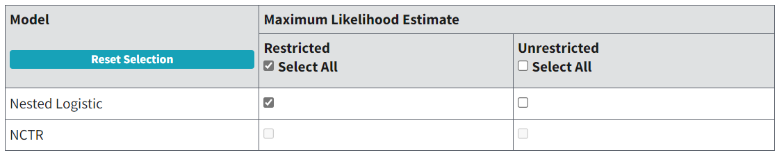
Figure 87. BMDS nested model selection.

Note

A third nested dichotomous model, the Rai and Van Ryzin model, can be accessed in BMDS 2.7, which is available from the BMDS website.

Entering Nested Dichotomous Data

A BMDS Online analysis can have a maximum of six datasets for nested dichotomous data.

For information on inserting or importing data, see Specifying Datasets.

The default column headers for nested dichotomous data are Dose, Litter Size, Incidence, and Litter Specific Covariate (LSC).

Note

There must be data in the LSC column even if the modeling options do not call for the use of LSC.

Figure 88. is a screenshot of a nested dataset in Excel that is formatted for use in BMDS.

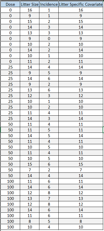
Figure 88. Nested dataset formatted correctly for BMDS analysis.

As Figure 88. shows, each litter is on a separate row, showing the dose it received, its sample size (Litter Size), the number of responders (Incidence), and the value of a covariate (Litter Specific Covariate).

Option Set

On the BMDS Online Settings tab, the user can define multiple Option Sets to apply to multiple user-selected models and multiple user-selected datasets in a single batch process. Select the blue Plus button to define a new Option Set configuration; select the red Trashcan icon to delete the Option Set.

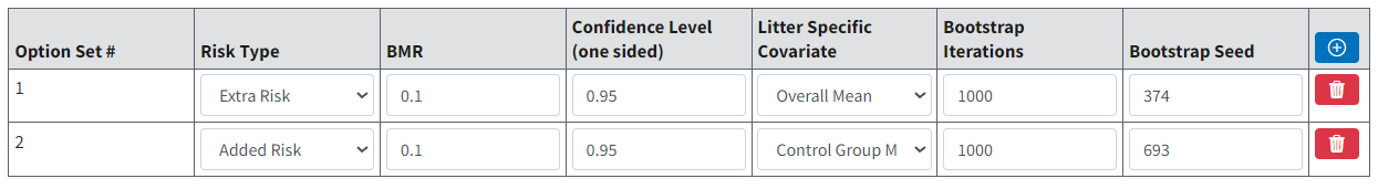
Figure 89. Nested Model options.

Risk Type

Choices for the Risk Type option are Extra Risk (default) or Added Risk.

Added risk is the additional proportion of total animals that respond in the presence of the dose, or the probability of response at dose \(d\), \(P(d)\), minus the probability of response in the absence of exposure, \(P(0)\):

\[added\ risk = P(d) –P(0)\]

Extra risk is the added risk divided by the proportion of animals that will not respond in the absence of exposure, \(1\ - \ P(0)\):

\[extra\ risk = \frac{P(d) –P(0)}{1 - P(0)}\]

Thus, extra and additional risk are equal when background rate is zero.

BMR

The BMR is the value of risk (extra or added, as specified by the user) for which a BMD is estimated. BMR must be between 0 and 1 (not inclusive). If \(P(0)\ > \ 0\), then values for BMR greater than \(1 - \ P(0)\) will result in an error when the risk type is added risk. That is because the maximum added risk that can ever be achieved is \(1 - \ P(0)\). In practice, this should not typically be an issue because one usually is interested in BMR values in the range of 0.01 to around 0.10.

BMR and Plots

The response associated with the BMR that is displayed in the graphical model output will only be the same as the BMR when \(P(0)\ = \ 0\).

This is because to obtain the actual response value one must solve for \(P(d)\) in the equation for added or extra risk discussed in Risk Type.

The horizontal bar depicting the response level used to derive the BMD that is displayed in the graphical model output will only be the same as the user-defined BMR (e.g., 10% Extra Risk) when the response at background, P(0), equals zero.

When P(0) does not equal zero, the true response level can be calculated using the Extra Risk equation described in Risk Type.

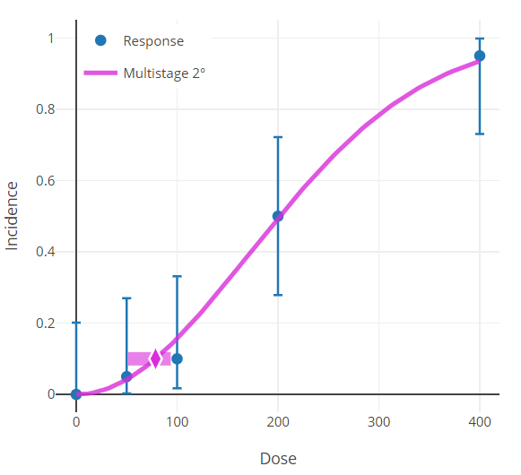
Figure 90. Results plot, with horizontal bar centered on the y-axis at the modeled BMR.

Confidence Level (one sided)

The Confidence Level is a fraction between 0 and 1; 0.95 is recommended by EPA (U.S. EPA, 2012).

The value for confidence level must be between 0 and 1 (not inclusive). For a confidence level of \(x\), BMDS will output BMDL and BMDU estimates, each of which is a one-sided confidence bound at level \(x\). For example, if the user sets the confidence level to 0.95 (the default), then the BMDL is a 95% one-sided lower confidence bound for the BMD estimate; the BMDU is a 95% one-sided lower confidence bound for the BMD estimate. In that example, the range from BMDL to BMDU would constitute a 90% confidence interval (5% in each tail outside that interval).

Litter Specific Covariate

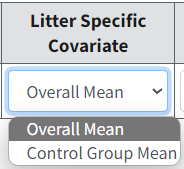
Figure 91. Litter Specific Covariate options.

Using a litter-specific covariate (LSC) enables the user to account for inter-litter variability.

Best practice would dictate not using a variable for the LSC if that variable is affected by dose (the other explanatory variable). During the analysis, it is recommended that the models with and without the LSC be compared to determine whether the LSC contributes to a better explanation of the observations (e.g., by comparing AIC values). For those runs where the LSC is included in the model, the BMD will depend on the LSC.

The Litter Specific Covariate option allows the user to determine if the BMD (and the corresponding plots) will be computed using the Control Group Mean value of the LSC or the Overall Mean value of the LSC (i.e., averaged across all dose groups; Overall Mean is the default selection). See BMD Computation for an explanation as to why this option is necessary, and which choice would be preferred for the given dataset.

The Overall Mean should be used under most circumstances. If the Litter-Specific Covariate differs from dose to dose (without any apparent consistent trend with respect to dose), consider using the Control Group Mean.

Note

Carr and Portier (Carr and Porter, 1991), in a simulation study, warn that in situations in which there is no effect of litter size, statistical models that incorporate a litter size parameter, as do the models in BMDS, will often erroneously indicate that there is a litter size effect. Thus, the user should use litter size parameters with caution. Unfortunately, there are currently no good diagnostics for determining whether a litter size effect exists.

Bootstrapping

Bootstrap Iterations: Specify the number of bootstrap iterations (default is 1000) to run to estimate goodness of fit. It is recommended to keep the value at a minimum of 1000. The maximum number of iterations is dependent on platform: in pybmds, the maximum is less than or equal to 1,000,000; in BMDS Online or BMDS Desktop, the maximum is less than or equal to 10,000.

Bootstrap Seed: BMDS auto-generates a seed for the random number generator by default. However, the user can specify a seed value, if needed for reproducibility.

For more details, refer to Bootstrap Results Table and Bootstrap Runs Table.

Specific Nested Dichotomous Results

Four Combinations of Nested Models

BMDS automatically runs all forms of the available nested models and displays the results on the Output tab. The codes following the model name indicate whether the litter specific covariate (lsc) and intralitter correlation (ilc) are included in the result.

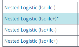
Figure 92. Nested model results as listed on the Output tab.

Table 7. All Forms of Nested Models run by BMDS

Litter Specific Coveriate	Intralitter Correlation - Estimated	Intralitter Correlation - Set to Zero
Inlcluded in Model	lsc+ilc+	lsc+ilc-
Not Included in Model	lsc-ilc+	lsc-ilc-

The Litter Specific Covariate is another variable that the model can (optionally) include, one that may help to explain the variation in the response from one experimental unit to another. The experimental unit is very often a litter of observations, hence the designation Litter Specific. For more details, refer to Litter Specific Covariate.

The intralitter correlation (again referencing the litter as a common experimental unit) variable estimates the degree to which observations within the same litter are correlated. If set to zero (one of the options), there is no correlation; the assumption then is that every observation is independent of every other observation (conditional on the model predicted probabilities of response).

Bootstrap Results Table

The nested models use a bootstrap approach for evaluating the fit of the model to the data under consideration. That approach takes the model with its MLE parameter values and simulates datasets matching the design (doses, sample sizes, etc.) being modeled. For each simulated dataset, the scaled residuals are computed and summed to yield a Chi-square test statistic. The distribution of that test statistic over the iterations is compared to the Chi-square test statistic from the observed data. If the model fits the data well, the observed Chi-square should not be in the upper tail of the Chi-square statistic values from the simulations. (For more on the Chi-square calculation, see Goodness-of-fit Information - Litter Data.)

The Bootstrap Results table summarizes the result of that test for goodness of fit. It reiterates the user-input number of iterations and displays the seed number used to generate the simulations (which may have been chosen randomly by BMDS). The log-likelihood and the Observed Chi-square test statistic pertain to the observed data. The Combined P-value can be used to infer whether the fit is adequate. Small p-values (e.g., less than 0.05 or 0.10) would indicate poor fit.

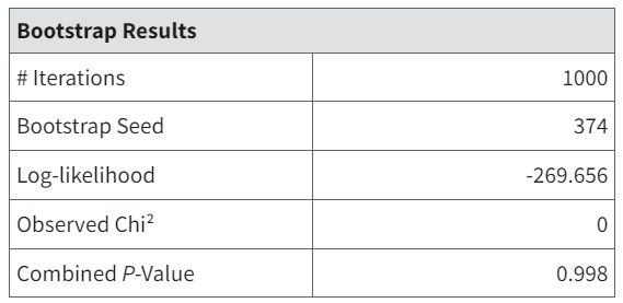
Figure 93. Bootstrap Results table.

Bootstrap Runs Table

The Bootstrap Runs table gives further details about the bootstrap test of fit. Since it is a random procedure (relying on random generation of datasets with the fitted model as the data-generating process) there is the possibility of noise entering into the computations.

Thus, BMDS runs the procedure three times and gets a p-value for each. These can be compared to determine if stability has been achieved. If not, the user may wish to increase the number of iterations.

Further details include middle and high-end percentiles for the Chi-square test statistic, that can be further compared to the observed value.

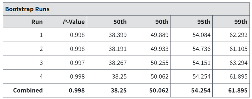
Figure 94. Bootstrap Runs table.

Scaled Residuals Table

In simple dichotomous modeling, there is a single scaled residual for each dose group. For nested designs, the probabilities of response and therefore the scaled residuals will vary across experimental units (i.e., litters). That variation is shown in the Litter Data table (Figure 96.) and summarized in the Scaled Residuals table (Figure 95.). The summary is an attempt to capture a general impression of the closeness of the observed response rates to those predicted by the model. As is typical, scaled residual values greater than 2 in absolute value may affect the user’s assessment of fit.

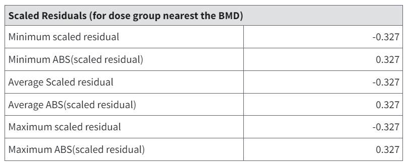
Figure 95. Summarized Scaled Residuals.

Note

Their are multiple values for scaled residuals reported in the Scaled Residuals table, including the minimum, average, and maximum scaled residual. The scaled residuals reported are the scaled residuals for the litters with litter specific covariate closest to the overall mean for the dose group closest to the estimated BMD. In the situation where there is only one litter with a litter specific covariate value closest to the mean value, the value reported for the minimum, average, and maximum scaled residual will be identical.

Litter Data Table

The Litter Data table shows the model-predicted probability of response and expected number of responders (i.e., \(Expected\ number\ of\ responders = Estimated\ Probability \times Litter\ Size\)).

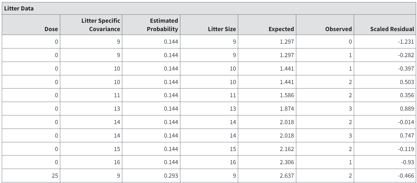
Figure 96. Partial capture of the Litter Data table.

Mathematical Details for Models for Nested Dichotomous Endpoints

The models that BMDS makes available for nested data are the Logistic Nested and NCTR models (see below). The user who is interested in the Rai and van Ryzin model is advised to download BMDS 2.7.

Individual Nested Dichotomous Models and their Respective Parameters

Nested Logistic model

Model Form

If \(dose > 0\)

\[p(dose) = {a + \theta}_{1}r_{ij} + \frac{(1 - \alpha - \theta_{1}r_{ij})}{(1 + e^{\left\lbrack - \beta - \theta_{2}r_{ij} - \rho \times \ln(dose) \right\rbrack})}\]

If \(dose = 0\)

\[p(dose) = \alpha + \theta_{1}r_{ij}\]

Parameters

\(\alpha\) = intercept (≥0)

\(\rho\) = power (≥0, can restrict to ≥1)

\(\beta\) = slope (≥0)

\(\theta_{1}\) = first coefficient for the litter specific covariate

\(\theta_{2}\) = second coefficient for the litter specific covariate

\(\phi_{1}, \ldots, \phi_{g}\) = intra-litter correlation coefficients

Notes

In the model equation, \(r_{ij}\) is the litter-specific covariate for the \(j^{th}\) litter in the \(i^{th}\) dose group. In addition, there are g intra-litter correlation coefficients; where g equals the number of dose groups.

\(0 \leq \phi_{i} \leq 1\ (i=1, \ldots, g)\)

\(1 > \alpha + \rho \geq \theta_{1}r_{ij} \geq 0\) for every \(r_{ij}\)

if \(r_{m}\) represents either the control mean value for the litter specific covariate or its overall mean, the BMD is computed as:

\[BMD = e^{\left\{ \frac{\left\lbrack \ln\left( \frac{A}{1-A} \right) - \beta - \theta_{2}r_{m}\right\rbrack}{\rho}\right\}}\]

where

\[\begin{split}A = \left\{ \begin{array}{r}\ BMRF\ extra\ risk \\ \\ \frac{BMRF}{(1 - a - \theta_{1}r_{m})}\ added\ risk\end{array} \right.\ \end{split}\]

For the BMDL, the parameter \(\beta\) is replaced with an expression derived from the BMD definition and the BMDL is derived as in BMDL Calculation

NCTR model

Model Form

\[p(dose) = 1 - e^{\left\{- (\alpha + \theta_{1}\left(r_{ij} - r_{m} \right)) - (\beta + \theta_{2}\left( r_{ij}-r_{m} \right)) \times dose^{\rho}\right\}}\]

Parameters

\(\alpha\) = intercept (≥0)

\(\rho\) = power (≥0, can restrict to ≥1)

\(\beta\) = slope (≥0)

\(\theta_{1}\) = first coefficient for the litter specific covariate

\(\theta_{2}\) = second coefficient for the litter specific covariate

\(\phi_{1}, \ldots, \phi_{g}\) = intra-litter correlation coefficients

Notes

In the model equation, \(r_{ij}\) is the litter-specific covariate for the \(j^{th}\) litter in the \(i^{th}\) dose group, \(r_{m}\) is the overall mean for the litter-specific covariate

\(\theta_{1}(r_{ij}-r_{m}) \geq 0\) and \(\theta_{2}(r_{ij}r_{m}) \geq 0\)

In addition, there are g intra-litter correlation coefficients; where g equals the number of dose groups.

\(0 \leq \phi_{i} \leq 1\ (i = 1, \ldots, g); 1 > \alpha + \rho \geq \theta_{1}r_{ij} \geq 0 \) for every \(r_{ij}\)

\[BMD = \left\lbrack \frac{- (\ln(1-A))}{(\beta + \theta_{2}\delta_{r})} \right\rbrack \times \left( \frac{1}{\rho} \right)\]

where

\[\begin{split}A = \left\{ \begin{array}{r}\ BMRF\ extra\ risk \\ \\ \frac{BMRF}{(1 - a - \theta_{1}\delta_{r})}\ added\ risk\end{array} \right.\ \end{split}\]

and \(\delta_{r}\) is the average of \(r_{ij}-r_{m}\) over either the control group of all observations (depending on user selection).

For the BMDL, the parameter \(\beta\) is replaced with an expression derived from the BMD definition and the BMDL is derived as in BMDL Calculation

Likelihood Function

Let \(g\) represent the number of dose groups. For the \(i^{th}\) dose group, there are \(n_{i}\) pregnant females administered dose \(dose_{i}\). In the \(j^{th}\) litter of the \(i^{th}\) dose group there are \(s_{ij}\) fetuses, \(x_{ij}\) affected fetuses, and, potentially, a litter-specific covariate \(r_{ij}\) which will often be a measure of potential litter size, such as number of implantation sites, though this is not a requirement of the models. In what follows, the dose-response model, which gives the probability that a fetus in the \(j^{th}\) litter of the \(i^{th}\) dose group will be affected, is represented by

\[p(dose_{i},\ r_{ij})\]

The beta-binomial distribution can be thought of as resulting from sampling in two stages. First, each litter is assigned a probability \(P_{ij}\) from a beta distribution (beta distributions represent a two-parameter family of probability distributions defined on the interval (0,1)). The parameters of the beta distribution are determined by the administered dose, the litter-specific covariate \(r_{ij}\) and the degree of intra-litter correlation, \(v_{i}\).

Note

The intra-litter correlation parameter varies among doses. It has been shown (Williams, 1988) that when the true intra-litter correlation differs among doses, unbiased estimates of the other parameters in a dose-response model can only be obtained if dose-specific intra-litter correlation parameters are estimated. As a special case, if \(v_{i} = 0\), then this part of the process is completely deterministic, and

\[P_{ij} = p(dose_{i},\ r_{ij})\]

This allows for the possibility of no litter effect at all.

In the second stage of sampling, \(s_{ij}\) fetuses are assigned to the litter, and the number of affected fetuses, \(x_{ij}\) is sampled from a binomial distribution with parameters \(P_{ij}\) and \(s_{ij}\).

The log-likelihood function that results from this process is (Kupper et al., 1986):

\[LL = \sum_{i = 1}^{g}\left\{ \sum_{j = 1}^{n_{i}}\left\lbrack \sum_{k = 1}^{x_{ij}}{ln(p\left( dose_{i},r_{ij} \right) + (k - 1)\Psi_{i}) + \sum_{k = 1}^{s_{ij} - x_{ij}}{\ln\left( 1 - p\left( dose_{i},r_{ij} \right) + (k - 1)\Psi_{i} \right) - \sum_{k = 1}^{s_{ij}}{ln(1 + (k - 1)\Psi_{i})}}} \right\rbrack \right\}\]

where

\[\Psi_{i} = \frac{\phi_{i}}{1 - \phi_{i}}\]

and

\[\sum_{a}^{b}{( \bullet ) = 0}\ if\ a > b\ (by\ convention).\]

This log-likelihood ignores a term that is independent of the values of the parameters.

Goodness of Fit Information Litter Data

The Litter Data table provides a listing of the data, expected and observed responses, and scaled residuals for each litter.

The scaled residual values printed at the end of the table are defined as follows:

\[\frac{(Obs\ - \ Expected)}{SE}\]

where Expected is the predicted number of responders from the model and SE equals the estimated standard error of that predicted number. For these models, the estimated standard error is equal to

\[\sqrt{\lbrack n \times p \times (1 - p) \times \left( \theta \times (n - 1) + 1 \right)\rbrack}\]

• \(n\) is the sample (litter) size,

• \(p\) is the model-predicted probability of response, and

• \(\theta\) is the model-predicted intra-litter correlation coefficient.

The overall model should be called into question if the scaled residual values are greater than 2 or less than -2 for several individual dose and litter-specific covariate combinations, particularly for the control group or a dose group near the BMD and for litter-specific covariate values close to the overall mean.

The goodness-of-fit p-values are calculated using a bootstrap approach.

1. The MLE parameter values are used to generate \(B\) pseudo-datasets having the same design features (number of doses and number of litters per dose), litter-sizes, and, if necessary, litter-specific covariate values, as the original dataset. What varies from pseudo-dataset to pseudo-dataset are the number of responding units within litters, and those are generated, at random, as dictated by the values of the ML estimates.

2. Once the B bootstrap iterations are generated, a statistic referred to as Chi-square is calculated for each. The Chi-square statistic is the sum of the squares of the scaled residuals for each litter, as described above. Higher values of that statistic are indicative of poorer match between the model predictions and the data.

3. The Chi-square statistic from the original data is computed and compared to the values from the \(B\) bootstrap iterations. The p-value is the proportion of Chi-square values from the iterations that are greater than the original Chi-square value.

High p-values are indicative of adequate fit (i.e., there was a high proportion of Chi-square values associated with pseudo-datasets obtained from data known to be consistent with the model and the ML estimates of the model parameters).

That calculation is repeated three times, and various percentiles of the generated Chi-square statistic are presented. This allows the user to determine if enough bootstrap iterations (B) have been specified. The default iterations for B is 1000 and should probably not be reduced. The user may wish to increase the default if the percentiles for Chi-square differ markedly across the three runs (specifically the median and lower percentiles), or if the p-values calculated from the three runs differ markedly. This may only be an issue when the p-value is close to the value (e.g., 0.05 or 0.10) used as a critical value for deciding if the fit of the model to the data is adequate. If there is some variability in the p-values, but they are all greater than 0.20, for example, then one probably need not worry about increasing the value for B.

Note

In traditional testing situations, the Chi-square statistic would be approximated by a Chi-square random variable having a certain degree of freedom, and its “significance” (p-value) would be determined from the appropriate Chi-square distribution function.

Plot and Error Bar Calculation

The error bars shown for the plots of nested data are calculated in the same way as those for dichotomous data (and described in Plot and Error Bar Calculation for dichotomous endpoints).

However, a Rao-Scott transformation is applied prior to the calculations to express the observations in terms of an effective number of affected fetuses divided by the total number in each group (the format required for the confidence intervals of simple dichotomous responses).

BMD Computation

BMD computation is like that for dichotomous models with the added wrinkle that a value for a litter-specific covariate (LSC) may be used, in addition to dose, to describe changes in the endpoint. It therefore affects the BMD calculation. If an LSC is included in the model, the user can choose to plot results and compute BMDs for one of two specific values of the LSC, either the overall mean (across all dose groups) or the control group mean. Typically, the overall mean is the preferred choice, but the control group mean might be appropriate in certain situations.

For example, suppose the LSC value varies enough from group to group to be “interesting,” but it goes up for some dose groups and down for others in a manner that does not indicate a dose effect. In this case, the user might decide to use the control group mean LSC when the BMD is close to the background dose (i.e., basically deciding that the LSC of interest in that region is more likely to be the average observed for the control group as opposed to the average across all the groups). If the LSC is found to be affected by dose (i.e., if its value appears to have a consistent trend with respect to dose), its use is discouraged.

Details of the BMD calculation are shown in Nested Dichotomous Models and their Respective Parameters.

BMDL Computation

BMDS currently only calculates one-sided confidence intervals, in accordance with current BMD practice. The general approach to computing the lower confidence limit for the BMD (called the BMDL here) is the same for all the models in BMDS, and is based on the asymptotic distribution of the likelihood ratio (Crump and Howe, 1985).

The approach used for all the nested dichotomous models is the same. The equations that define the benchmark response in terms of the benchmark dose and the dose-response model are solved for one of the model parameters, using either the control group mean or the overall mean of the litter-specific covariate. The resulting expression is substituted back into the model equations, with the effect of re-parameterizing the model so that BMD appears explicitly as a parameter. A value for BMD is then found such that, when the remaining parameters are varied to maximize the likelihood, the resulting log-likelihood is less than that at the maximum likelihood estimates by exactly

\[\frac{\chi_{1,1 - 2\alpha}^{2}}{2}\]