TADA R8 Demo January 2026
TADA Team
2026-07-07
Source:vignettes/TADAWorkFlowDemoR8.Rmd
TADAWorkFlowDemoR8.RmdOverview and Setup
Welcome!
Thank you for your interest in Tools for Automated Data Analysis (TADA). TADA is an open-source tool set built in the R programming language. This RMarkdown document walks users through how to download the TADA R package from GitHub, access and parameterize several important functions, and create basic visualizations with a sample data set.
Note: TADA is still under development. New functionality is added weekly, and sometimes we need to make bug fixes in response to tester and user feedback. We appreciate your feedback, patience, and interest in these helpful tools.
If you are interested in contributing to TADA development, more information is available at:
We welcome collaboration with external partners.
Install and load packages
First, install and load the remotes package specifying the repo. This is needed before installing TADA because it is only available on GitHub.
install.packages("remotes",
  repos = "http://cran.us.r-project.org"
)
library(remotes)
Next, install and load TADA using the remotes package. TADA R Package dependencies will also be downloaded automatically from CRAN with the TADA install. You may be prompted in the console to update dependency packages that have more recent versions available. If you see this prompt, it is recommended to update all of them (enter 1 into the console).
remotes::install_github("USEPA/EPATADA",
  ref = "develop",
  dependencies = TRUE
)
Finally, use the library() function to load the TADA R Package into your R session.
Help pages
All TADA R package functions have their own individual help pages, listed on the Function reference page on the TADA GitHub site. Users can also access the help page for a given function in R or RStudio using the following format (example below): ?[name of TADA function].
# Access help page for TADA_DataRetrieval
?TADA_DataRetrieval
A) Retrieving, filtering and cleaning data from the WQP
Query the WQP using TADA_DataRetrieval. TADA_AutoClean is a powerful function that runs as part of TADA_DataRetrieval when applyautoclean = TRUE. It performs a variety of tasks, for example:
creating new “TADA” prefixed columns and and capitalizing their contents to reduce case sensitivity issues,
converts special characters in value columns,
converts latitude and longitude values to numeric,
replaces “meters” with “m”,
replaces deprecated characteristic names with current WQX names,
harmonizes result and detection limit units,
harmonizes depth units to meters, and
creates the column TADA.ComparableDataIdentifier by concatenating characteristic name, result sample fraction, method speciation, and result measure unit.
In this example, we will get dissolved oxygen concentration, Escherichia coli, and pH data from January 2020 to December 2022 (two years) from Missoula County, Montana. Then we will run the following three functions:
TADA_RunKeyFlagFunctions is a shortcut function to run
important TADA flagging functions. See ?function documentation for
TADA_FlagResultUnit, TADA_FlagFraction, TADA_FlagMeasureQualifierCode,
and TADA_FlagSpeciation for more information.
Censored data are measurements for which the true value is not known,
but we can estimate the value based on known lower or upper detection
conditions and limit types. TADA fills missing
TADA.ResultMeasureValue and
TADA.ResultMeasure.MeasureUnitCode values with values and units
from TADA.DetectionQuantitationLimitMeasure.MeasureValue and
TADA.DetectionQuantitationLimitMeasure.MeasureUnitCode,
respectively, using the TADA_AutoClean function. The TADA
package currently has functions that summarize censored data incidence
in the dataset and perform simple substitutions of censored data values,
including x times the detection limit and random selection of a value
between 0 and the detection limit. The user may specify the methods used
for non-detects and over-detects separately in the input to the
TADA_SimpleCensoredMethods function. In this example, no
censored data results were found.
The TADA_HarmonizeSynonyms function converts synonymous
data to a unified naming format for easier aggregation, analysis, and
visualization.
Data_MT_MissoulaCounty <- TADA_DataRetrieval(
  startDate = "2020-01-01",
  endDate = "2022-12-31",
  statecode = "MT",
  characteristicName = c("Escherichia", "Escherichia coli", "pH"),
  countycode = "Missoula County",
  ask = FALSE
) |>
  TADA_RunKeyFlagFunctions() |>
  TADA_SimpleCensoredMethods() |>
  TADA_HarmonizeSynonyms()
Rename the Data_MT_MissoulaCounty data frame to tada.MT. Generate a table:
# Assign it to tada.MT
tada.MT.clean <- Data_MT_MissoulaCounty

# Optionally, remove the original dataset from the environment
rm(Data_MT_MissoulaCounty)

# Generate a table
TADA_TableExport(tada.MT.clean)
Flag, clean, and visualize
Now, let’s use EPATADA functions to review, visualize, and whittle the returned WQP data down to include only results that are applicable to our water quality analysis and area of interest.
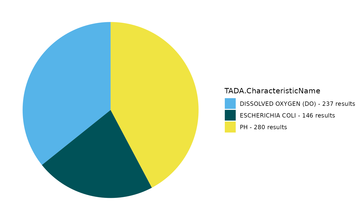
Create a pie chart to display the count of results for each TADA.CharacteristicName.
TADA_FieldValuesPie(
  tada.MT.clean,
  field = "TADA.CharacteristicName",
  characteristicName = "null"
)
TADA is primarily designed to accommodate water data from the WQP. Let’s see what activity media types are represented in the data set.
Are there any media types that are not water?
# Create table with count for each ActivityMediaName
media <- TADA_FieldValuesTable(
  tada.MT.clean,
  field = "ActivityMediaName"
)

DT::datatable(media, fillContainer = TRUE)
Create an overview map. For each site, we can view the measurement count, visit count and characteristic counts along with the site ID, site name, and organization name.
TADA_OverviewMap(tada.MT.clean)Let’s take a quick look at all unique values in the MonitoringLocationIdentifier column and see how how many results are associated with each.
# use TADA_FieldValuesTable to create a table of the number of results per MonitoringLocationIdentifier
sites <- TADA_FieldValuesTable(
  tada.MT.clean,
  field = "MonitoringLocationIdentifier"
)

DT::datatable(sites, fillContainer = TRUE)
What about OrganizationFormalName?
# use TADA_FieldValuesTable to create a table of the number of results per MonitoringLocationIdentifier
orgs <- TADA_FieldValuesTable(
  tada.MT.clean,
  field = "OrganizationFormalName",
)

DT::datatable(orgs, fillContainer = TRUE)
TADA_FindQCActivities identifies results with QA/QC
identifies results with QA/QC ActivityTypeCodes. When clean = TRUE, it
removes QA/QC results.
tada.MT.clean <- TADA_FindQCActivities(tada.MT.clean, clean = TRUE)The functions TADA_FlagAboveThreshold and TADA_FlagBelowThreshold are used to flag results falling above and below the WQX national thresholds, respectively. When clean = TRUE, the flagged results are removed from the TADA data frame.
tada.MT.clean <- TADA_FlagAboveThreshold(tada.MT.clean, clean = TRUE, flaggedonly = FALSE)

tada.MT.clean <- TADA_FlagBelowThreshold(tada.MT.clean, clean = TRUE, flaggedonly = FALSE)
B) Create an Assessment Unit/WQP Monitoring Location crosswalk.
The TADA_CreateAUMLCrosswalk function
efficiently creates a crosswalk between ATTAINS assessment units and WQP
monitoring locations. It uses three prioritized data sources:
User-Supplied Crosswalk: An optional crosswalk provided by the user (e.g., see example
user.supplied.cwin next code chunk).ATTAINS Crosswalk: Utilizes
TADA_GetATTAINSAUMLCrosswalkto incorporate crosswalk information stored by participating organizations in ATTAINS. There may not be an ATTAINS crosswalk available for all organizations as storing this information in ATTAINS is optional for states and some tribes are still in the process of developing their crosswalks.ATTAINS Catchments/Geospatial Join: Employs
TADA_CreateATTAINSAUMLCrosswalkto connect monitoring locations to assessment units using ATTAINS catchments through a geospatial join. This function converts WQP monitoring locations into a geospatial sf object and associates them with their intersecting NHDPlus high resolution catchments containing entity-defined assessment units in ATTAINS.
Process
- The function prioritizes these sources in the order listed. It automatically attempts to assign unassigned monitoring locations using the next available data source. For example, if any monitoring locations remain unassigned after checking the user-supplied crosswalk, the function will check the ATTAINS crosswalk, then the geospatial join, as needed.
For demonstration purposes, let’s assume we know for sure this MonitoringLocationIdentifier, “MTWTRSHD_WQX-COMBITR02” should be associated with the AssessmentUnitIdentifier “MT76M001_020”. Let’s create a crosswalk to assign “MTWTRSHD_WQX-COMBITR02” to the assessment unit “MT76M001_020” and give it the WaterType “RIVER”.
Get Expert Query API Key
Some aspects of this workflow depend on ATTAINS data imported via Expert Query web services. While public, Expert Query web services require an API key, a unique identifier used to authenticate access to the Expert Query API. The EPATADA package contains a default API key for Expert Query, so users who do not have their own API key can still use these functions.
However, Expert Query API keys are rate limited, meaning that if many users are all accessing Expert Query data using the same key at the same time, server failures from too many requests may occur. Best practice is for each EPATADA user is to obtain their own, individual API key by requesting one here: API Key Signup Form
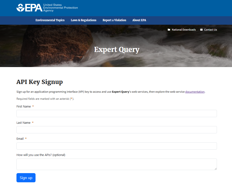
If you have your own API key, uncomment the code below and assign your API key to the “api_key” variable. Otherwise, the default EPATADA package key will be used.
# api_key <- "paste your key here"

# is user does not provide key, set api_key as NULL
if (!exists("api_key")) {
  api_key <- NULL
}
Define a user supplied crosswalk of Assessment Units and Monitoring Location(s)
# user would like to associate this MonitoringLocationIdentifier to this AU.
user.supplied.cw <- data.frame(
  AssessmentUnitIdentifier = "MT76M001_020",
  MonitoringLocationIdentifier = "MTWTRSHD_WQX-COMBITR02",
  WaterType = "RIVER"
)

DT::datatable(user.supplied.cw, fillContainer = TRUE)
Run TADA_GetATTAINSCrosswalk
Now, let’s check to see if MTDEQ has submitted a prior crosswalk to ATTAINS for the assessment unit identifier “MT76M001_020”.
Does our TADA data frame contain any of these monitoring locations?
ATTAINS.cw <- TADA_GetATTAINSAUMLCrosswalk(
  org_id = "MTDEQ",
  api_key = api_key
) |>
  dplyr::filter(ATTAINS.AssessmentUnitIdentifier == "MT76M001_020")

any(unique(tada.MT.clean$MonitoringLocationIdentifier) %in% ATTAINS.cw$ATTAINS.MonitoringLocationIdentifier)
Run TADA_CreateAUMLCrosswalk
We are uncertain about any other assignments of assessment units to monitoring locations. Let’s match the monitoring locations catchments overlay from tada.MT.clean with assessment units catchments with a geospatial join from ATTAINS by using TADA_CreateATTAINSAUMLCrosswalk to identify which assessment units intersect with each monitoring location.
Recall, TADA_CreateATTAINSAUMLCrosswalk prioritizes the user supplied crosswalk, user.supplied.cw. If any monitoring locations remain unassigned after checking the user-supplied crosswalk, the function will check the ATTAINS crosswalk (see ATTAINS.cw above), then lastly, the geospatial join, as needed.
# make AU assignments for unassigned MLs
MT.AUMLRef <- TADA_CreateAUMLCrosswalk(tada.MT.clean,
  au_ref = user.supplied.cw,
  org_id = "MTDEQ",
  fill_ATTAINS_catch = TRUE,
  return_nearest = TRUE,
  batch_upload = FALSE,
  api_key = api_key
)
The output of TADA_CreateAUMLCrosswalk is a list of data frames: 1)
“TADA_with_ATTAINS”
2) “ATTAINS_catchments”
3) “ATTAINS_points”
4) “ATTAINS_lines” 5) “ATTAINS_polygons”
6) “ATTAINS_crosswalk”
The data frame, TADA_with_ATTAINS contains all of the clean TADA data as well as the added ATTAINS columns. The other ATTAINS_catchments, ATTAINS_points, ATTAINS_lines, and ATTAINS_polygons data frames contain geometry for mapping. The ATTAINS_crosswalk data frame contains a simple crosswalk of monitoring locations and assessment units.
Now, let’s view the assessment units and monitoring locations on a map to review the assessment unit/monitoring location assignments.
TADA_ViewATTAINS(MT.AUMLRef, ref_icons = TRUE)C) Assigning uses to assessment units.
Let’s filter our TADA data frame to a single assessment unit “MT76M001_020”, and for a single TADA.CharacteristicName, “DISSOLVED OXYGEN (DO)” for demonstration purposes for the remainder of this example.
# get subset DO data for one AU
tada.MT.clean.DO <- MT.AUMLRef$TADA_with_ATTAINS |>
  sf::st_drop_geometry() |>
  dplyr::filter(
    TADA.CharacteristicName == "DISSOLVED OXYGEN (DO)",
    ATTAINS.AssessmentUnitIdentifier == "MT76M001_020"
  )

tada.MT.AUMLRef <- MT.AUMLRef$ATTAINS_crosswalk |>
  dplyr::filter(ATTAINS.AssessmentUnitIdentifier == "MT76M001_020")
Retrieve Uses from Prior ATTAINS Assessment Cycles
Let’s retrieve the use names assigned to this example assessment unit from a prior ATTAINS assessment cycle for MTDEQ. Users can append additional rows or remove use names as needed. See the TADA Module 2: Geospatial Functions vignette for more information.
AU.uses <- TADA_AssignUsesToAU(
  tada.MT.clean.DO,
  org_id = "MTDEQ",
  AUMLRef = tada.MT.AUMLRef,
  api_key = api_key
)

TADA_TableExport(AU.uses)
From a User Supplied Crosswalk (Uses to AU)
Users may also choose to supply their own list of use names if desired rather than sourcing it from the prior ATTAINS assessment cycle. To ensure we use the correct column names, we can run TADA_AssignUsesToAU() with no argument function inputs. Note: The TADA.AssessmentUnitStatus column is auto populated and does not need to be supplied from a user supplied crosswalk.
For ATTAINS.WaterType, please ensure this matches the ATTAINS.WaterType from the output of MT.AUMLRef$ATTAINS_crosswalk for your assessment unit.
names(TADA_AssignUsesToAU())

AU.uses.user.supplied <- data.frame(
  ATTAINS.OrganizationIdentifier = c("MTDEQ", "MTDEQ"),
  ATTAINS.AssessmentUnitIdentifier = c("MT76M001_020", "MT76M001_020"),
  ATTAINS.UseName = c("Example: Aquatic Life, cold waters", "Example: Human Health"),
  ATTAINS.WaterType = c("RIVER", "RIVER"),
  IncludeOrExclude = c("Include", "Include")
)

AU.uses2 <- TADA_AssignUsesToAU(
  tada.MT.clean,
  org_id = "MTDEQ",
  AUMLRef = tada.MT.AUMLRef,
  AU_UsesRef = AU.uses.user.supplied,
  api_key = api_key
)

TADA_TableExport(AU.uses2)
D) Create a TADA-compatible Criteria and Methodologies Table
The EPATADA Module 3 functions are being designed to:
- Assist users with creating a Criteria and Methodologies table,
- Analyze Water Quality Portal results using the user supplied Criteria and Methodologies table.
Users can choose to:
- Fill in and populate their own criteria table manually,
- use an auto_assign method of creating a crosswalk of ATTAINS parameter names to WQX Characteristic and to CST pollutant names along with a crosswalk between ATTAINS use names and EPA Criteria Search Tool (CST) uses. This allows for populating the magnitude components from the CST for each ATTAINS parameter and use, if one is found for your organization (duration, frequency and other methodology components will still need user inputs and a thorough review of the crosswalk between the CST and ATTAINS parameter and uses will be required),
- or pull in their organization’s criteria table from a list of pre-filled templates from the TADACommunityHub* if one exists (currently all R8 states and tribes have participated in submitting their organization’s criteria table to this repository!).
* The TADACommunityHub is a collaborative hub where TADA users share and maintain information for custom workflows (e.g., state, tribal, territory, EPA, or other entities). For example, it includes user-contributed criteria and methodologies templates to support reproducible and efficient analyses.
The EPA 304A criteria and methodologies are also available for use.
TADA Community Hub Criteria and Methodologies Templates
For this demo, We will load in a pre-filled criteria template for MTDEQ (draft). The reference tables may need additional review by the region and states/tribes.
# Load the example R8 criteria table for MTDEQ
criteria_table <- TADA_ListCriteriaFile(org_id = "MTDEQ")

MT_criteria <- TADA_DefineCriteriaMethodology(
  tada.MT.clean.DO,
  org_id = "MTDEQ",
  criteriaMethods = criteria_table,
  AUMLRef = tada.MT.AUMLRef,
  AU_UsesRef = AU.uses,
  displayUniqueId = TRUE
)

TADA_TableExport(MT_criteria)
Assistance with Generating a Criteria and Methodologies Template from Scratch
Alternatively, if your organization has not submitted a criteria table to the TADACommunityHub repository, TADA_DefineCriteriaMethodology has an auto_assign function input which allows populating the magnitude values from the Criteria Search Tool (CST) to past ATTAINS.ParameterName and ATTAINS.UseName for your organization from prior submission to ATTAINS assessment cycles. Filter it to just “DISSOLVED OXYGEN (DO)”.
Note that duration, frequency and other criteria components will still need to be filled out with auto_assign. However, if users are only interested in individual result measurement excursions, they can proceed to use this table as is.
criteria_table_auto <- TADA_DefineCriteriaMethodology(
  tada.MT.clean,
  org_id = "MTDEQ",
  auto_assign = T,
  criteriaMethods = NULL,
  AUMLRef = tada.MT.AUMLRef,
  AU_UsesRef = AU.uses,
  displayUniqueId = TRUE
) |>
  dplyr::filter(TADA.CharacteristicName == "DISSOLVED OXYGEN (DO)")

TADA_TableExport(criteria_table_auto)
We will continue using the criteria table for MTDEQ that was submitted to the TADACommunityHub.
Editing the criteria table in excel
If further edits are desired to the criteria table, users can export the criteria table into an excel spreadsheet and read it back into the R environment once any edits are made.
MT_criteria_excel <- TADA_DefineCriteriaMethodology(
  tada.MT.clean.DO,
  org_id = "MTDEQ",
  criteriaMethods = criteria_table,
  AUMLRef = tada.MT.AUMLRef,
  AU_UsesRef = AU.uses,
  displayUniqueId = TRUE,
  excel = T,
  overwrite = T
)
View and analyze scatter plot excursions for DO for assessment unit
Now, lets view some scatter plots for the criteria defined in your criteria table which will be compared to the results from your TADA data frame for DO for a single assessment unit, “MT76M001_020”. We will join your TADA data frame to the criteria table using the MTDEQ table sourced from the TADACommunityHub.
# join use and criteria to tada df (many to many relationships may occur)
tada.MT.clean.DO2 <- dplyr::left_join(
  tada.MT.clean.DO,
  MT_criteria,
  by = "TADA.ComparableDataIdentifier"
)

# break into separate data frames for each unique combination of DurationValue, DurationMethod, DurationUnit, and UniqueSpatialCriteria for analysis and figures
tada.MT.do.subsets <- tada.MT.clean.DO2 |>
  dplyr::group_by(
    DurationValue, DurationMethod, DurationUnit,
    UniqueSpatialCriteria
  ) |>
  dplyr::group_split()
Note that the scatter points are only individual result measurements. The TADA Team is working on developing functions for handling the criteria (magnitude, duration and frequency) and methodologies information (e.g. seasonality and data sufficiency) entered into the Criteria and Methodologies Template.
TADA_scatters <- list()

n <- length(tada.MT.do.subsets)

for (i in 1:n) {
  # need to set this up as function to plot multiple
  desc <- paste0(
    "Lower bound for ",
    tada.MT.do.subsets[[i]]$ATTAINS.UseName[1],
    " (",
    tada.MT.do.subsets[[i]]$DurationValue[1],
    " ",
    tada.MT.do.subsets[[i]]$DurationUnit[1],
    " ",
    tada.MT.do.subsets[[i]]$DurationMethod[1],
    " for ",
    tada.MT.do.subsets[[i]]$UniqueSpatialCriteria[1],
    ")"
  )

  TADA_scatters[[i]] <- TADA_Scatterplot(tada.MT.do.subsets[[i]]) |>
    plotly::add_lines(
      x = c(
        min(tada.MT.do.subsets[[i]]$ActivityStartDate, na.rm = TRUE),
        max(tada.MT.do.subsets[[i]]$ActivityStartDate, na.rm = TRUE)
      ),
      y = (tada.MT.do.subsets[[i]]$MagnitudeValueLower[1]),
      inherit = FALSE,
      name = paste(strwrap(desc, width = 20), collapse = "<br>"),
      line = list(color = "red", dash = "dash")
    )

  names(TADA_scatters)[i] <- desc
}
The criteria and methodologies table for DO contained multiple rows. Let’s view the different options and explore which might be appropriate for our assessment unit.
Here is what the scatter plots might look like if the “Lower bound for Aquatic Life (1 n-day arithmetic min for Cold water, other life stages present)” and “Lower bound for Aquatic Life (7 n-day arithmetic mean for Cold water, other life stages present)” criteria and methodologies information was determined to be the appropriate criteria for this assessment unit and applied.
names(TADA_scatters)
# TADA_scatters
TADA_scatters[[1]]
TADA_scatters[[5]]